November 19, 2019
Investment Theory
Negative Interest Rates and the Perpetuity Paradox
By Victor Haghani and James White 1
“We are actively competing with nations who openly cut interest rates so that now many are actually getting paid when they pay off their loan, known as negative interest. Who ever heard of such a thing? Give me some of that. GIVE ME SOME OF THAT MONEY. I WANT SOME OF THAT MONEY.”
– President Donald Trump, Economic Club of New York, November 12, 2019
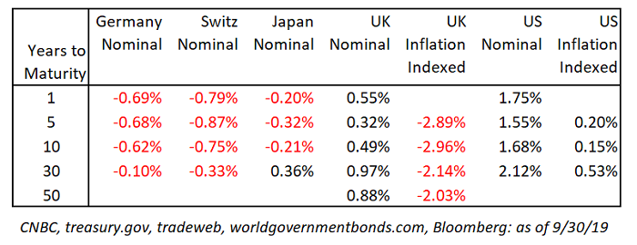
If President Trump had his way, the US would be sporting significantly negative rates right now. While there is wide-ranging disagreement on the long-term impact of negative interest rates 2 – good, bad or neutral – there is growing acceptance that negative interest rates are the ‘new normal’ with 30% of the world’s government bonds trading at sub-zero yields, as illustrated in the table below.
Negative Rates and Ultra-Long-Term Bonds
For Wall Street’s bond-pricing models, negative interest rates mostly have been no big deal; the same code usually works just fine when yields are negative instead of positive.3 But there is at least one exception, a bond type that cannot abide a negative yield: the Consol bond.4 Even though governments don’t issue them anymore, they’re one of the simplest and oldest of all bonds. Also known as Perpetuities, these bonds provide the holder with a fixed interest payment each year in perpetuity. They were issued and re-issued by governments such as the UK, France and the US, and were often the market’s largest and most actively-traded issues. The UK retired their last Consol bonds in 2015, and today there are virtually no government-issued perpetual bonds outstanding. However, there are plenty of other perpetual or near-perpetual cash flow streams investors can buy, and recently issued sovereign bonds with maturities of 50 to 100 years may feel like near-perpetual offerings to many investors.
The basic formula for the price of a perpetual is simple:
p = c y
where symbols represent price, coupon and yield, for y > 0 .
Two noteworthy aspects of the formula: 1) for any positive coupon and positive finite price, the perpetuity cannot have a negative yield, and 2) price approaches infinity as the yield of the perpetuity approaches zero.
The chart below illustrates the relationship between the price and yield of a perpetuity and annuities with different maturities. Notice how extremely convex these curves become at very low interest rates. This kind of convexity is generally an attractive characteristic for buyers of such investments, and a terrifying one for short-sellers.
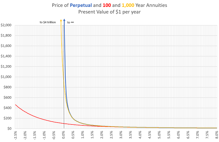
To avoid having to deal directly with infinity – clearly a price that no-one would be willing or able to pay – we’ll consider a 1,000-year annuity paying $1 per year, rather than a Perpetuity. If we know interest rates are fixed for the next 1,000 years, we can easily calculate and see the annuity’s price on the chart above, but what’s a reasonable fair price given some uncertainty in interest rates? Let’s approximate this value by imagining 1,000 different interest-rate scenarios. Let’s say that, in 999 scenarios, interest rates will equal 2%. But in just one scenario, we’ll assume rates will instead average -1%, in the spirit of the ‘new-normal’ for interest rates and the possibility that interest rates can be negative for sustained periods of time in the future. The Expected Value of the annuity is the probability-weighted average of the Values of the annuity that result from those scenarios, producing a result which is pretty remarkable:
| 99.9% probability of 2% rates; annuity value of $50 |
| 0.1% probability of -1% rates; annuity value of $2,316,257 (!) |
| Expected Value of the annuity is $2,366, which is a yield of -0.15%.5 |
A Potential Perpetuity Paradox
What we’re calling the Perpetuity Paradox is the conundrum facing a person who simultaneously believes that there’s a small chance negative interest rates can persist for long periods of time, but would not pay a price anywhere close to the $2,366 Expected Value of the annuity for more than a de minimis amount. We are not claiming that most people hold these beliefs…but if you do (and we don’t think it’s unreasonable to do so) then you’ve got a paradox on your hands.
One solution to this potential paradox is suggested by the resolution to the St. Petersburg Paradox, proposed by Daniel Bernoulli in 1738. The St. Petersburg Paradox involves a game that no one would pay much to play, despite the game having an infinite Expected Value. The common thread in both the Perpetuity Paradox and the St. Petersburg Paradox is that what someone will be willing to pay is, in the absence of riskless arbitrage, often determined by their Expected Utility and not the Expected Dollar Value of the gamble.6
In working with Expected Utility, we’re going to assume a level of risk aversion typical of 30 of our investors we surveyed a year ago. We find that even at a price of just $51 for the annuity a typical investor would optimally invest only 1/2000th (0.05%) of her wealth, even though the price represents a 98% discount to Expected Value.7 Much closer to the Expected Value of $2,366, a price of $2,100 merits an optimal investment of only 1/10,000th (0.01%) of wealth. Thus, we can see the Expected Utility line of reasoning presents one resolution to the ‘paradox’: even though the small possibility of negative rates makes the ‘gamble’ on the annuity highly valuable, an ordinary investor wouldn’t bet more than a tiny fraction of wealth on it. Sadly, the UK government can forget about issuing one 1-Pound-per-year inflation-indexed Perpetuity to pay off the entire national debt!
Conclusion
We can’t say how long the new-normal of negative interest rates will continue – but given the negative long-term nominal and real rates we see in a number of major economies, it seems difficult to dismiss negative rates as just a fleeting phenomenon. That means it’s worth seriously thinking through the issues involved in valuing and investing in long-lived cash-flow streams, whether arising from government bonds, real estate or equities, near and below the zero interest rate frontier.
Regardless of your position on negative interest rates, we hope this note has illustrated two important and intriguing considerations that impact many important investment decisions under uncertainty:
- Convexity matters: The Expected Value of long-term cash flows is highly convex, especially in the region of low discount rates. It’s noteworthy, in this case, how only a tiny assumed probability of negative rates has such an enormous impact on Expected Value.
- Utility matters more: Supply and demand is what sets prices, and in the absence of arbitrage, Expected Utility trumps Expected Value in assessing how much demand investors will have for an investment.
Appendix: Using a Probabilistic Interest Rate Model to Put a Value on a Near-Perpetuity
It’s hard to describe how far-out the idea of negative interest rates has been to economists and market participants throughout history. What would Sidney Homer, co-author of the 4,000 year survey “A History of Interest Rates” and Salomon Brother’s first director of Bond Research, have made of UK investors’ locking in a 65% loss in the purchasing power of their savings by buying 50-year inflation-linked bond at a yield of -2.03%? 8 Influential economists and philosophers through the ages, including Marshall, Fisher, von Mises, Hicks, Hayek, Knight, Keynes and Friedman, all wrote books and articles proposing differing theories of interest rates. One common thread was that none of them envisioned negative interest rates as a realistic phenomenon they needed to explain.
It wasn’t until the late 1970s that economists started to directly embed uncertainty and randomness into interest rate models, thereby taking account of the convexity of discounted cash flows so central to the Perpetuity Paradox we’re discussing. Since then, many stochastic interest rate models have been proposed, including those by Vasicek (1977), Cox-Ingersoll-Ross (1985), Heath-Jarrow-Morton (1989), Black-Derman-Toy (1990) and White-Hull (1990, 2006). For the case at hand, simplicity and familiarity persuaded us to use a model similar to one that we used at Salomon Brothers, called the 2+ model, in the days when banks were allowed to invest their own capital in proprietary trading.9
We’ll use this model to generate 1,000 possible paths for future interest rates, which in turn produce bond prices and corresponding yields. We’ll parameterize the model so that the expected bond prices are roughly consistent with the pricing of German bonds with maturities of 1, 5, 10 and 30 years, taken from Table 1.
Below is a description of the model. An important feature is that it allows the short-term interest rate to go as negative as h:
dx = ƛ dt + 𝞂1 dw1
dy = -ɣ y dt + 𝞂2 dw2
dz = -k (z – x – y)dt
r = ez – h
The chart below shows the value of a $1 a year 1,000-year annuity for each of 1,000 paths we generated with this model, arranged from smallest to largest value, and plotted on a log scale since some of the values are so large.
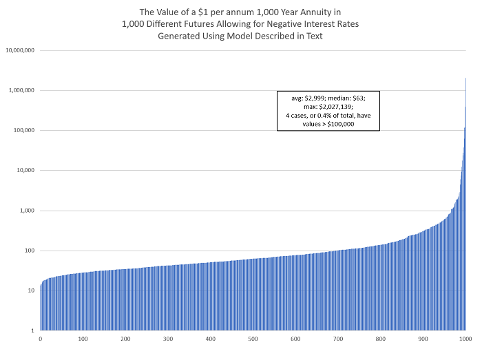
You can see how the Expected Value of the annuity is heavily influenced by a small number of very large expected dollar values, just as we suggested in our two-scenario analysis in the body of the note. This is the distribution of values of the 1,000-year annuity which are consistent with the current market pricing for German government bonds, taking into account the uncertainty around future interest rates and the possibility that interest rates stay negative for prolonged periods, consistent with the new-normal perspective.
As noted above, we are using a no arbitrage model of interest rates for this analysis. This means that in theory, if the 1,000 year annuity were trading at a price below the model price, an arbitrageur could buy it and hedge it with other bonds and make a riskless profit equal to the difference between the market and model price of the annuity. There are significant limitations involved in doing this in practice for such a long horizon asset, including transactions costs and frictions in holding the required highly leveraged long and short positions of the hedge portfolio, the necessity of the particular interest rate model chosen to have a form and parameterization which accurately describes how interest rates evolve in the future and the extremely long horizon involved in forcing convergence to the model.
Alternative interest rate models will produce charts that can look substantially different than the one above. For example, models that assume interest rates will mean-revert to a fixed and pre-known positive level will not produce paths that put such high values on the annuity, but then we’d suggest that such models are not really in the spirit of the new-normal for interest rates. As discussed above, we believe that Expected Utility analysis is the best tool for figuring out what an individual would be willing to pay for this distribution of outcomes, and thereby resolves the apparent paradox of perpetuity pricing in a future that may experience negative interest rates for sustained periods.
Update:
Bloomberg author Brandon Kochkodin wrote a great piece in response to our post on negative interest rates, which you can read by clicking the link below:
How Negative Rates Can Send Bond Prices Soaring
Victor also took a moment to talk about negative rates on BloombergTV, watch the full interview below:
Further Reading and References
- Black. F.. E. Derman and W. Toy. “A One-Factor Model of Interest Rates and Its Application to Treasury Bond Options.” Financial Analysts Journal. 1990.
- Cochrane. John. “A New Structure for U.S. Federal Debt.” Hoover Institution. working paper. May 2015.
- Cochrane, John. “Why Stop at 100? The Case for Perpetuities.” The Grumpy Economist. August 2019.
- Cox, J.C., J.E. Ingersoll and S.A. Ross. “A Theory of the Term Structure of Interest Rate.” Econometrica. 1985.
- Dybvig, Philip, Jonathan Ingersoll and Stephen Ross. “Long Forward and Zero-Coupon Rates Can Never Fall.” Journal of Business. 1996.
- Heath, David, Robert Jarrow and Andrew Morton. “Bond Pricing and the Term Structure of Interest Rates: A New Methodology for Contingent Claims Valuation.” Econometrica. 1992.
- Homer, Sidney and Richard Sylla. “A History of Interest Rates.” Wiley Finance. 1963.
- Hull, John and Alan White. “Pricing interest-rate derivative securities.” The Review of Financial Studies. 1990.
- Vasicek, O. “An equilibrium characterization of the term structure.” Journal of Financial Economics. 1977.
- Saeedy, Alexander. “100 Year Bonds? Why ‘Ultra-Long’ Bonds Have Caught on in 14 Countries and Counting.” Fortune. August 2019.
- LePan, Nicholas. “The History of Interest Rates Over 670 Years.” Visual Capitalist. November 2019.
- This not is not an offer or solicitation to invest. Past returns are not indicative of future performance.
Thank you to Simon Bowden, John Cochrane, Emanuel Derman, Rich Dewey, Ian Hall, Larry Hilibrand, Costas Kaplanis, Bob Kopprasch, Vlad Ragulin, Jeff Rosenbluth, and Rob Stavis for their comments and suggestions.
- We’ll use the term ‘interest rates’ to refer to both nominal and real (inflation-adjusted) interest rates, except where we think it’s useful to make a distinction. And, we’ll use ‘yield’ and ‘yield to maturity’ to refer to the IRR which discounts a set of bond cash-flows to a given price.
- Negative interest rates do imply an arbitrage for investors who can keep cash under the mattress, but this generally doesn’t apply to institutional investors. For investors lacking sufficient mattress space, simple interest rates also need to be greater than -100%, or else borrowing money would be an arbitrage – you would get paid today to receive $1 in the future. Interest rate derivative models have also required modifications to allow for negative interest rates.
- Originally short for ‘Consolidated Annuity.’
- Notice the big difference between the Expected Value of the annuity, and the value of the annuity at the Expected Yield. The Expected Yield of the annuity is 1.997% (99.9% chance it’s 2% and 0.1% chance it’s -1%). The value of the annuity at the Expected Yield of 1.997% is $50, whereas as shown here the Expected Value of the annuity is $2,366. The difference is due to the convexity of the price as a function of the yield of the annuity.
- This puzzle is also reminiscent of the Mega Millions lottery that we discussed about a year ago, when we suggested that, ignoring the fun value involved, even a ticket with an Expected Value far in excess of its price warrants only a tiny investment by a risk-averse investor.
- We assume the risk-free asset earns 0%, and that the investor views owning the perpetuity as a risky gamble to be determined by which interest-rate environment is ‘drawn’ from the distribution. If the investor viewed the 1000-year annuity as her minimum-risk asset of choice, she would want to own substantially more than suggested by this analysis, and we’d need to look elsewhere to resolve this paradox.
We assume the investor displays Constant Relative Risk Aversion (CRRA) with a coefficient of risk aversion of 2.5, about average from our survey. Such an investor would be indifferent to a gamble with a 50/50 chance of a 40% gain or 20% loss in wealth. In the Appendix, we present a slightly expanded analysis using a term-structure model, but we feel that what the above analysis lacks in rigor, it makes up for in simplicity.
- Very roughly, assuming the bond has a 0% coupon (it actually has a 0.125% coupon), the calculation is 1 – (1 – 2.03%)50 = 64% .
- A 1996 paper by Dybvig, Ingersoll and Ross, titled “Long Forward and Zero-Coupon Rates Can Never Fall,” discusses the asymptotic behavior of interest rates as time to maturity goes to infinity, and makes a case based on no arbitrage for why long forward rates cannot continually fall. We believe the behavior of long forward rates arising from the 2+ model presented here does not violate the no arbitrage constraint.