December 11, 2019
Investment Theory
Mind the Gap: Inequality and Diversification
By Victor Haghani, Jeffrey Rosenbluth and James White 1
Introduction
Understanding the origins of wealth inequality is critical in the debate over what, if anything, to do about it. In this note, we propose a simple model which is still rich enough to reproduce observed patterns of wealth inequality. We call it the Concentrated Asset Betting (CAB) model. A key element of CAB is a phenomenon known in the gambling world as “over-betting the edge.” Our approach was inspired by Bruce Boghosian’s Scientific American article “Is Inequality Inevitable?” which provides an introduction to a straightforward model of wealth inequality called the “Yard Sale Model” (YSM).
In a Yard Sale model, it is assumed that people enter into repeated exchanges with each other. In each exchange one party is chosen at random to be the “winner” and one the “loser.” The absolute size of the exchange is determined by the assets of the less wealthy party. As the number of exchanges increases, the model converges to one person having all the money in the economy. To match observed levels of wealth inequality in different countries at different times, the YSM is then extended to include wealth redistribution and a couple of other enhancements.
Model Description
The model we propose is based on the observation that a high fraction of investors have experienced sub-par growth in their savings, after allowing for consumption and philanthropy, relative to the tremendous long-term growth in the public stock market. Victor presented some anecdotal evidence of this in his TEDx talk, “Where Are All the Billionaires and Why Should We Care?” Some of the reasons put forward to explain the shortfall in investor returns include investment fees, commissions and taxes. Our model suggests there may be something even larger and more insidious at work – pervasive and systematically poor money management. Here, money management means the task of sizing and diversifying the risks of a portfolio of investments.
Numerous academic studies have documented the tendency of investors to hold significantly undiversified portfolios, especially in the pre-Vanguard era up to the early 1990s. With commissions of $70 or more per trade, investors had an incentive to minimize the number of individual stocks they held.2 A study by Vanguard observed that from the 1950s through the 1980s investors’ equity exposure came almost entirely through directly-held stocks, and the median investor held only two stocks.3
The most basic version of our model begins with a population of households all with the same initial wealth. Each household starts off fully-invested in one stock.4 If their wealth increases, they increase the number of stocks they own, thereby increasing their diversification. We add one stock to their portfolio each time their wealth doubles. Each portfolio is split equally among however many stocks they own, rebalancing monthly.
Every stock has an annual expected return of 6%, which roughly matches the US stock market’s annual price appreciation over the past hundred years.5 We assume a 19% standard deviation of monthly returns, consistent with Hendrik Bessembinder’s large-scale study “Do Stocks Outperform Treasury Bills?” For simplicity, we assume the stocks are uncorrelated with each other.6
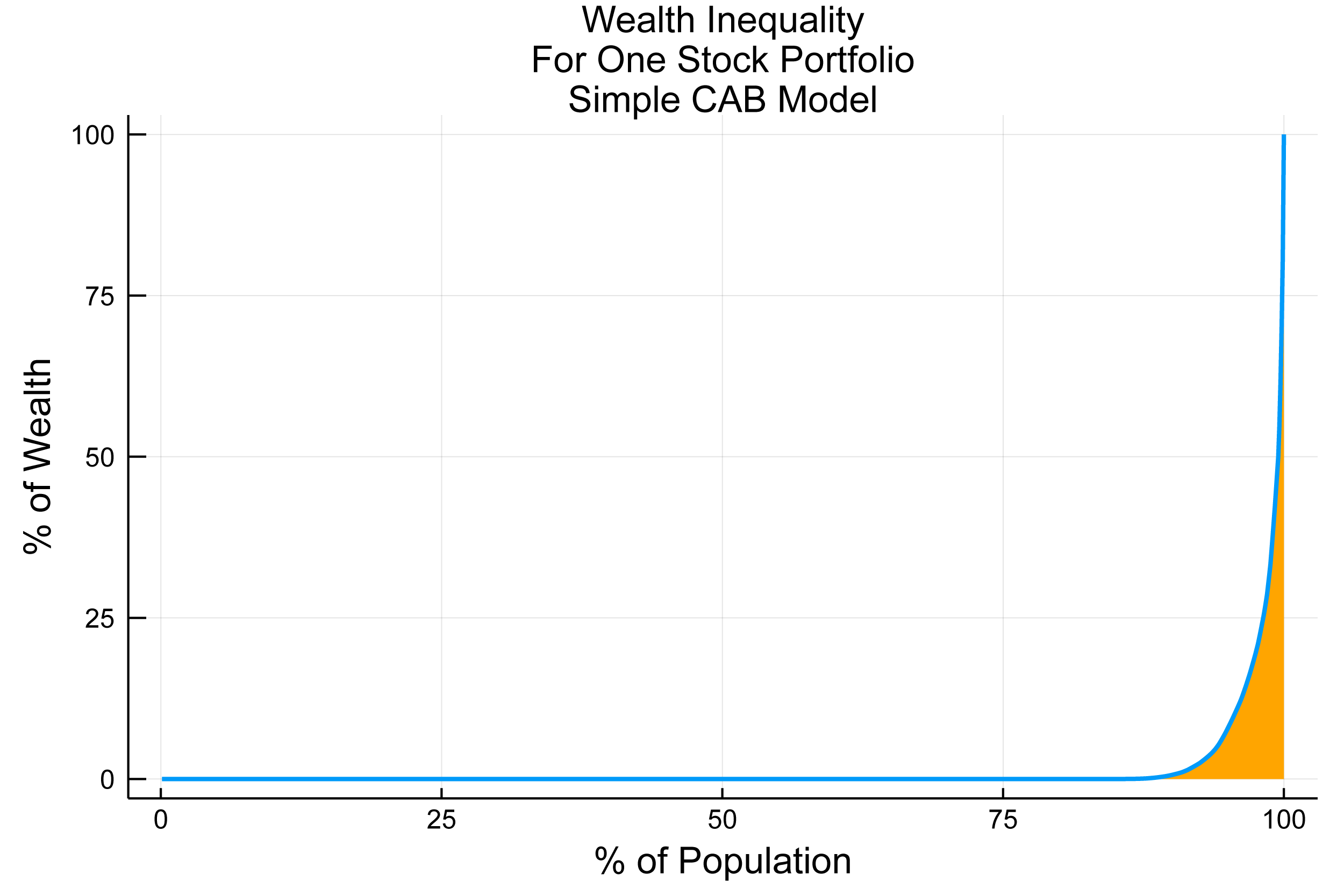
In our simulation, we flip a coin for each stock every month. If heads, the stock in question gains 19.5%. If tails, it loses 18.5%. This gives us the desired 19% standard deviation, with monthly expected return of 0.5% (6% annualized) for each individual stock.7 The chart below shows the ending wealth distribution after running this simulation for 100 years on 1000 families. Like the YSM, our model predicts a high level of wealth inequality. Unlike the YSM, our model features a growing economy.
Interpreting Model Results
All families have identical prospects starting out, yet high levels of wealth inequality naturally arise anyway. What’s at work here? First, with portfolios concentrated in just a few individual stocks, chance creates a lot of inequality in wealth outcomes.8 Second, good luck, measured by the number of heads flipped, translates into increasingly large incremental gains in wealth. That means wealth as a function of luck is highly convex in the long-term, as good or bad luck compounds multiplicatively rather than additively. This can be seen in the dramatic curvature of wealth plotted against number of heads flipped over 100 years in the chart below.
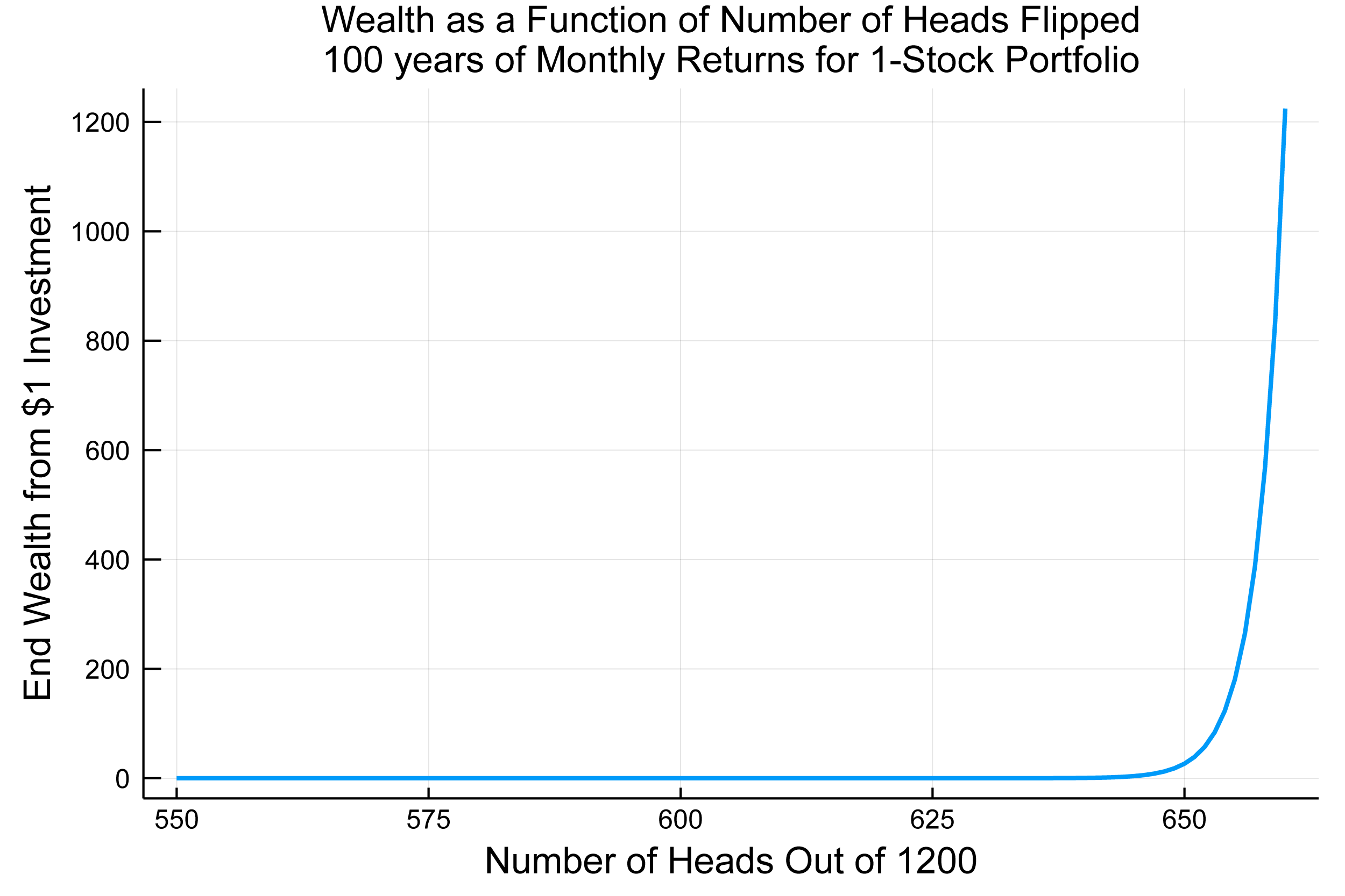
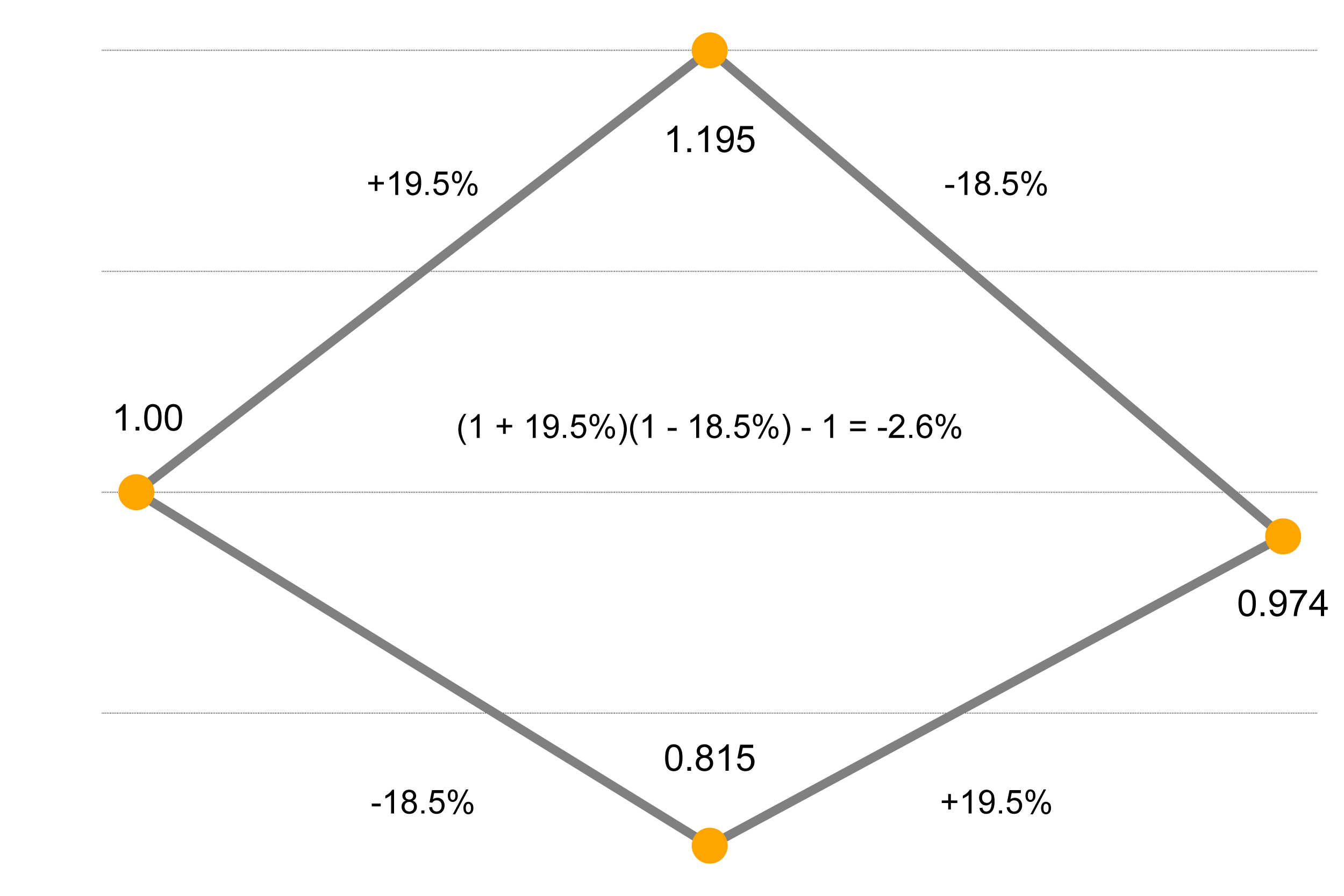
The third force leading to extreme inequality causes many families to wind up with near zero wealth despite investing in stocks that are all expected to rise 6% a year, as can be seen in the chart above. Over the 1,200 months of the 100-year simulation, the expected number of heads is 600, half of the total flips. Yet, the chart shows that if a household experienced 600 heads, they’d wind up with close to 0 wealth. In fact, they need to get 642 heads just to break even.9 This results from “over-betting the edge,” defined as taking so much risk that you lose money in the central case of flipping an equal amount heads and tails. If a single stock portfolio gains 19.5% one month and then loses 18.5% the next month, the total return over the two months is not the +1% you’d get from two months of +0.5% expected return per month. Rather, it is -2.6% as illustrated in the diagram below.10
In addition to being able to generate different levels of inequality to a given horizon, we can also influence the degree of wealth mobility in our system by choosing how quickly we allow families to diversify their portfolios by adding more stocks with increases in a household’s wealth. Through this mechanism, the winners get more diversification, lessening their over-betting and increasing the chance of keeping and growing their winnings.
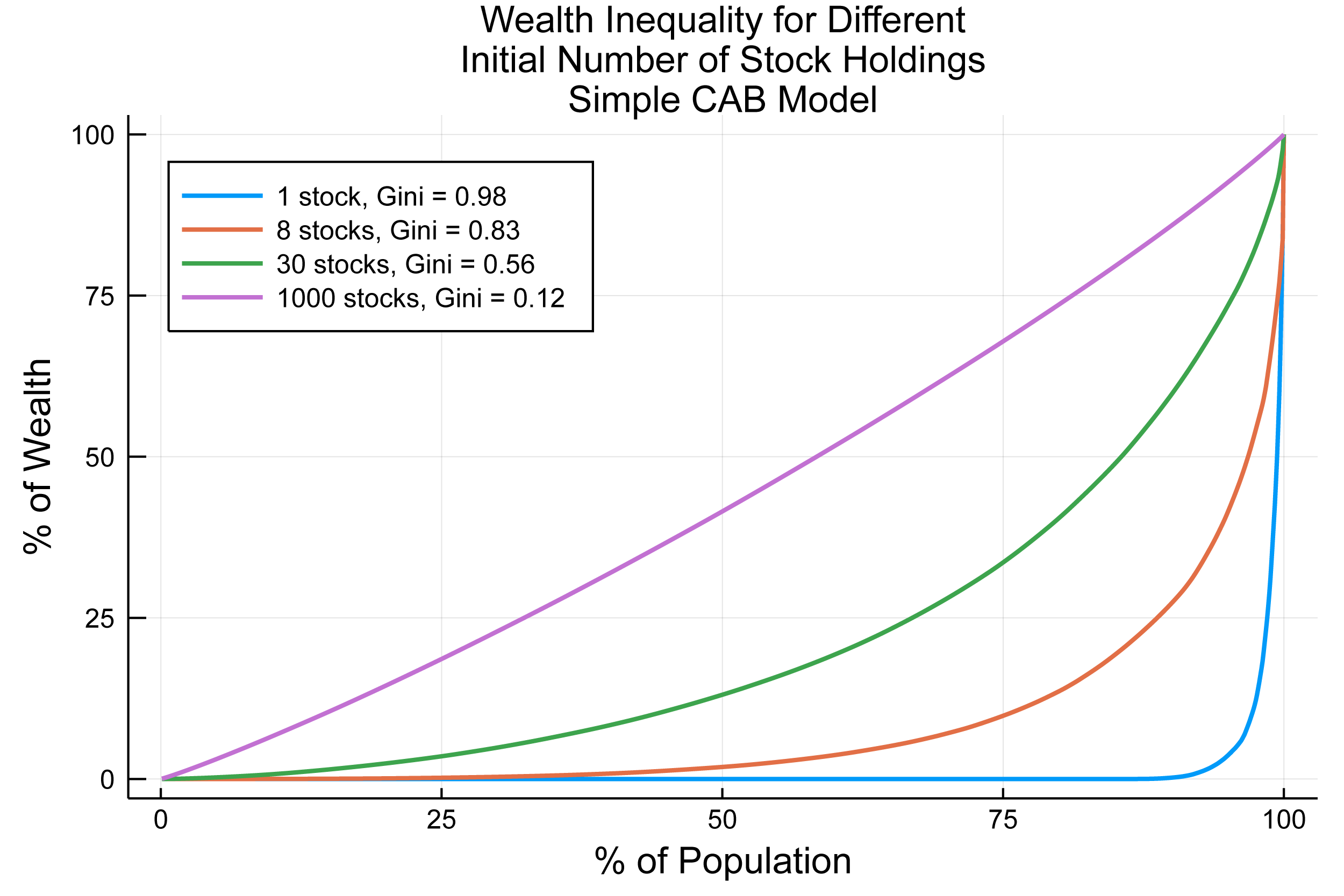
An important parameter in the basic form of our model is the number of stocks initially held. The chart below shows how greater initial diversification, and thus less over-betting, dramatically lessens wealth inequality. For each distribution of wealth curve, we calculate the Gini coefficient, a popular summary metric of inequality.11 Holding 100% of wealth in an 8-stock portfolio represents the acceptable amount of risk for a gambler who bases her risk-taking on the Kelly Criterion, a commonly-used metric which gamblers generally agree sets an upper bound on how much risk to take for a given opportunity.12 Even though an investor with an 8-stock portfolio in our framework can no longer be accused of over-betting, she could still improve the quality of her portfolio dramatically with more diversification. If we had investors start off with portfolios of 1,000 stock holdings, we’d get very little wealth inequality, which is what we’d expect if most families held the market portfolio through an index fund.
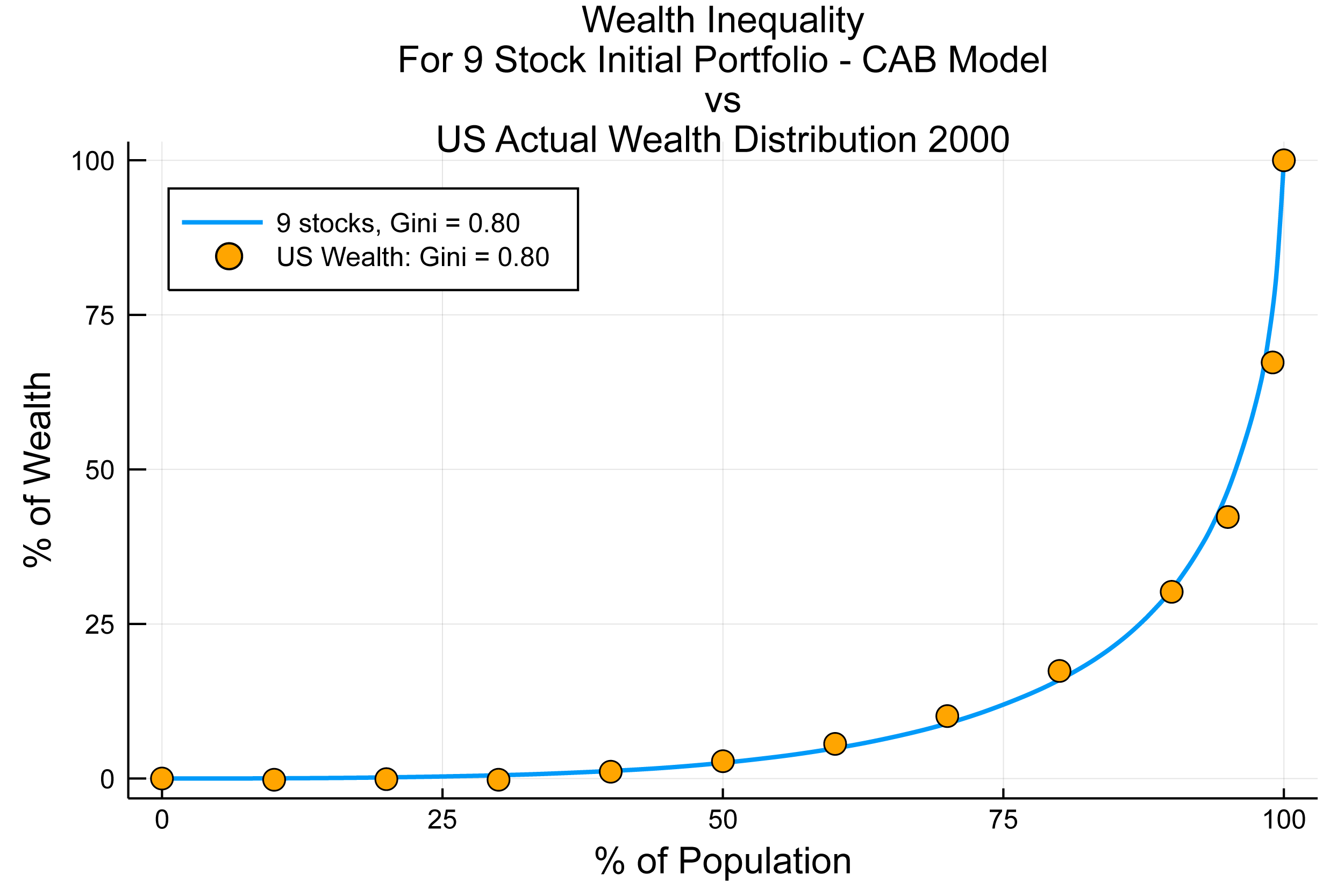
The chart below displays the actual distribution of wealth in the US in 2000,13 which is a good fit with our model using a 9-stock initial portfolio for each investor.
Conclusions and Future Research
While we recognize that there are many causes of wealth inequality, the CAB Model provides a simple and empirically-supported explanation for how the level of wealth inequality seen today came about. Some of the assumptions we’ve made may seem extreme by today’s standards, such as using a 19% monthly standard deviation of stock returns, but the CAB results are robust to more moderate assumptions. Indeed, if the US investing scene for most of the 20th century resembles developing markets today, then a recent paper by Campbell et al, “Do the Rich Get Richer in the Stock Market? Evidence from India (2018),” provides direct support for the CAB explanation of wealth inequality resulting from pervasive under-diversification.14
We hope this short note will spur further research focused on understanding the properties of this model of wealth inequality, and on refinements to make the model more realistic while still retaining its parsimonious structure. In particular, we hope to explore its ability to match observed levels of wealth mobility, the impact of a wealth-redistribution tax, and how to incorporate non-participation and underinvestment in risky assets as another important cause of long-term wealth inequality.
The CAB model provides an alternative to that proposed by Thomas Piketty in “Capital in the 21st Century” (2014), which assumes that equity returns are high and constant, so once a household gets rich enough to have significant investable wealth, they’re going to get richer and richer.15 Unlike Piketty’s Capital model, CAB tells us where the “missing billionaires” may have gone, incorporates pervasive sub-optimal risk sizing, and predicts the frequently observed downward mobility of the undiversified wealthy. It also points the way to a more level potential distribution of wealth in the future, due to the growth over the past 20 years of index funds and other diversified mutual funds.16
Unlike the Piketty and the Yard Sale models, the CAB paradigm does not see extreme wealth inequality as an inevitable and convergent feature of “pure” capitalism absent specific offsetting policies such as wealth redistribution. Rather, it shines a bright and hopeful light on one possible path to less wealth inequality in the future, which is for investors to think more carefully about diversification and investment-sizing, thus improving their chances of participating in the long-term expected wealth creation opportunities offered by public markets.
Further Reading and References
- Angle, John. “The surplus theory of social stratification and the size distribution of personal wealth.” Social Forces, pp. 293–326. 1986.
- Barber, Brad, and Terrance Odean. “Trading Is Hazardous to Your Wealth:The Common Stock Investment Performance of Individual Investors.” Journal of Finance. April 2000.
- Bessembinder, Hendrik. “Do Stocks Outperform Treasury Bills?” Journal of Financial Economics. 2017.
- Bessembinder, Hendrik, Te-Feng Chen, Goeun Choi and K.C. John Wei. “Do Global Stocks Outperform US Treasury Bills?” SSRN. 2019.
- Boghosian, Bruce. “Is Inequality Inevitable?” Scientific American. November 2019.
- Calvet, Laurent, John Y. Campbell and Paolo Sodini. “Down or Out: Assessing the Welfare Costs of Household Investment Mistakes.” Journal of Political Economy, Vol. 115, No. 5, pp. 707-747. 2007.
- Campbell, John Y., Tarun Ramadorai and Benjamin Ranish. “Do the Rich Get Richer in the Stock Market? Evidence from India.” SSRN. 2018.
- Chakraborti, Anirban. “Distributions of money in model markets of economy.” International Journal of Modern Physics, pp. 1315–1321. 2002.
- Clarke, Andrew, Michael Nolan and Tyrone Sampson. “What is a Mutual Fund Worth?” Vanguard Research. October 2019.
- Davies, James, Susanna Sandström, Anthony B. Shorrocks and Edward N. Wolff. “The Level and Distribution of Global Household Wealth.” NBER Working Paper No. 15508. 2009.
- Haghani, Victor, Jeffrey Rosenbluth and James White. Concentrated Asset Betting. 2019.
- Hayes, Brian, “Follow the Money.” American Scientist 90, pp. 400–405, 2002.
- Li, Jie, Bruce M. Boghosian and Chengli Li. “The Affine Wealth Model: An agent-based model of asset exchange that allows for negative-wealth agents and its empirical validation.” arXiv.org. 2016.
- Wood, Geoffrey and Steve Hughes. “The Central Contradiction of Capitalism? A collection of essays on Capital in the Twenty-First Century.” Policy Exchange. 2015.
- US Wealth Distribution Data from Federal Reserve: Distributional Financial Accounts.
- This not is not an offer or solicitation to invest. Past returns are not indicative of future performance.
Thank you to John Campbell, Larry Hilibrand, Steven Landsburg, and Vlad Ragulin for their very helpful comments and guidance.
- Schwab historical commissions.
- Clark et al, 2019:
“In the early 1950s, 4.2% of the U.S. population participated in the stock market, almost entirely through directly held stocks (Federal Reserve Board, 2019). These investors held undiversified portfolios – a median of two stocks. Half held one stock…Stock investing resembled a game of portfolio roulette. In today’s terms, one spin of the wheel might come up Amazon. The next might be Enron. This approach predominated until the 1980s.”
- We assume there are enough stocks so that each household owns different stocks.
- We are in effect assuming that each household spends the dividends they receive on their stock portfolio.
- It may appear that the assumption that the individual stocks are uncorrelated, and hence all have a Beta of 0, is unrealistic. Relaxing that assumption, for example by giving all stocks a Beta of 1, does not materially change our results.
- As will become apparent below, even if we had chosen a single stock risk level half of the Bessembinder estimate, the model would produce a similar pattern of results.
- The wealth inequality among families generated in our simple model is a direct reflection of the highly unequal long-term performance of individual common stocks, which is partly a result of the compounding effect we described above. Bessembinder (2017) observes that:
“…approximately 26,000 stocks that have appeared in the CRSP database since 1926 are collectively responsible for lifetime shareholder wealth creation of nearly $32 trillion dollars. However, the eighty six top-performing stocks, less than one third of one percent of the total, collectively account for over half of the wealth creation. The 1,000 top performing stocks, less than four percent of the total, account for all of the wealth creation…The positive skewness arises both from the fact that monthly returns are positively skewed, and from the possibly underappreciated fact that compounding introduces positive skewness into the multi-period return distribution even if single period returns are distributed symmetrically…which contributes to the concentration of wealth creation.”
- But if they get just 18 heads more than that, for a total of 660 heads, their wealth will have grown more than one-thousand-fold, catapulting them into the ranks of the super-rich. Unfortunately, there is only 0.03% probability of getting 660 or more heads.
- By contrast, a one-stock portfolio with just 15% invested in the single stock would make money in the central case of flipping an equal number of heads and tails, i.e.. (1 + 15% * 19.5%) (1 – 15% * 18.5%) – 1 = +0.07% . The Kelly Criterion calls for 14%, rather than the 15% in this example, and anything over 28% (i.e. twice the Kelly bet) would be over-betting as we’ve defined it here.
- The Gini Coefficient on Wikipedia.
- The Kelly Criterion on Wikipedia.
- Davies, James, Susanna Sandström, Anthony B. Shorrocks and Edward N. Wolff. “The Level and Distribution of Global Household Wealth.” NBER Working Paper No. 15508. 2009.
- The authors conclude:
“Return heterogeneity increases the inequality of account size through two main channels, both of which are related to the prevalence of undiversified accounts that own relatively few stocks. The first is that some undiversified portfolios randomly do well, while others do poorly. The second is that larger accounts tend to earn higher average log returns. They do so not by earning higher average simple returns, but by limiting uncompensated idiosyncratic risk which lowers the average log return for any given average simple return.” (p15). - See this paper for a set of essays evaluating the Piketty model:
“The Central Contradiction of Capitalism? A collection of essays on Capital in the Twenty-First Century,” Edited by Geoffrey Wood and Steve Hughes (2015). - See Calvet et al (2007) for how Swedish households at the turn of the 21st century were making better investment decisions, but still with room for material improvement, than Americans were for most of the 20th century.