September 4, 2018
How Elm Works
Tax Efficiency and Dynamic Asset Allocation: Can We Have Our Cake and Eat It Too?
By Victor Haghani and James White 1
We are frequently asked about the tax efficiency of our dynamic value-and-momentum investment approach. The concern is often that with estimated turnover of 50% – 100% per year, returns might be less tax-efficient than a simple static, buy-and-hold type of approach, which is generally recognized as the gold-standard of tax-efficient investing.2 As we’ll explain below, we believe our dynamic approach is expected to be, and has been, as tax-efficient as a static one.
In this note, we will:
- describe the historical tax-efficiency of our approach, as experienced by an actual investor for the past six years. In the Appendix, we show simulated results for the past 11 years, and…
- explain why we expect to continue to deliver tax-efficiency in US taxable portfolios, particularly through the inherently favorable tax characteristics of momentum-induced rebalancing and from the account-by-account, tax-aware portfolio-rebalancing tools we’ve developed in-house.
Tax-Efficiency of an Elm Investor (2012-2017)
While tax performance in a particular instance will strongly depend on the specific path of the market and the investor’s entry and exit point(s),3 the actual experience of one of our early investors may be a useful illustration of the degree of tax-efficiency we can deliver.4 The example below is from an investor in our Delaware Fund. While our Fund is different in a number of material ways from an SMA account, we chose this example as it allows us to share a history twice as long as what we have for SMAs.5 We have also run longer-term comparative simulations based on investment start dates from 2007 to the present, with results consistent with the example we show here – see the Appendix for details. As always, we emphasize that even ten years of historical experience, in and of itself, cannot tell us much about what to expect in the future.6
In the table below, we compare the income and its tax character from our chosen investor versus a simulated fixed-weight portfolio with the same Baseline weights as Elm’s strategy,7 and rebalanced back to those weights each month.
| Actual Investment in Elm Fund | Static Fixed Weight Asset Allocation | Tax Rate: Approximate Allocation |
|
| Start Value: Jun. 1, 2012 | $10,000,000 | $10,000,000 | |
| End Value: Dec. 31, 2017 | $15,540,340 | $15,095,500 | |
| Increase in Investment | $5,540,340 | $5,095,500 | |
| Unrealized Capital Gains | $3,644,880 | $3,164,590 | 15% |
| Total Realized Capital Gains | $298,700 | $291,924 | |
| Short-term Capital Gains (Losses) | ($459,360) | $45,243 | 41% |
| Long-term Capital Gains | $758,060 | $246,681 | 24% |
| Qualified Dividends | $867,580 | $848,738 | 24% |
| Int Inc & non-Qualified Dividends | $610,850 | $629,692 | 41% |
| Tax-exempt Income | $118,330 | $160,556 | 0% |
| Blended Tax Rate on Investment | 17.1% | 18.8% | |
| Past returns and tax characteristics may not be indicative of future returns and tax character. Note: summarized k-1 data: e.g. foreign tax credits and misc deductions are not shown separately. |
|||
The right-most column displays the assumed Federal tax rate applied to each type of income. Notice that we use 15% for unrealized capital gains, 9% lower than the 24% for realized long-term capital gains, in recognition of the benefits of deferring capital gains tax.8 If we applied an 18% rate to unrealized gains for the dynamic strategy and 15% for the static strategy, to reflect the higher expected turnover of the dynamic strategy in the future, this would increase the blended tax rate of the dynamic strategy by 1.9%, putting it roughly in line with the static approach.
Bottom line: not only did our chosen investor do over 4% better than a simulated static weight investor on a pre-tax total return basis (with about 10% lower risk),9 but, over a reasonable range of assumptions, he experienced an effective blended tax rate that was attractive in absolute terms, and also was roughly equal to, or possibly even lower than, that of a static weight investor.10
Elements of a Tax-Aware Approach
Over this period, if our Fund had rebalanced exactly back to our desired asset allocation each month, turnover would have averaged about 80% per year, while the static, fixed weight approach would have experienced turnover of just 14% per year. However, in practice, both turnover rates would be lower as neither strategy would be rebalanced exactly back to target each month.
Despite the higher turnover of Elm’s strategy, there are several subtle but significant effects that together yield high expected (and so far, realized) tax-efficiency for our dynamic approach. First, the momentum overlay is what generates most of the additional turnover compared to a static approach. Its nature is to generate frequent but small short-term capital losses punctuated by less frequent but large long-term capital gains. Second, our portfolio turnover generally takes the form of buying and selling a small ‘top’ slice of the portfolio, which typically has relatively low built-up gains or losses. Beneath this ‘top’ slice, there will tend to be a more static base layer of the portfolio that can hold a buildup of unrealized long-term capital gains. Keeping track of specific tax lots also contributes to greater tax efficiency. Finally, a substantial fraction of total income is generally in the form of tax-preferred Qualified Dividends and tax-exempt municipal bond income, a benefit enjoyed by both the dynamic and static-weight strategies.11
In addition to the features described above, which relate to Elm’s core asset-allocation strategy, we apply additional tax-aware portfolio management techniques at the execution level. Our rebalancing algorithm recommends the transactions that will achieve the best trade-off between minimizing realized gains, minimizing transaction costs, maximizing realized losses, and staying close to our asset-allocation targets.12 Because many of the dozen or so markets we invest in are related, and several different instruments are generally available per market, we can often achieve a much better tax result for our investors than if we naively re-balanced each market exactly to target without thinking about taxes. Our taxable investors also benefit from periodic tax-loss harvesting, and our system automatically works to prevent tax-adverse wash sales between groups of linked accounts.
Conclusion
We hope this admittedly-limited treatment of this important topic sheds some light on our ability to deliver tax efficient returns through a systematic, dynamic and tax-aware asset allocation approach. We put a lot of focus on tax-efficiency, just as we do on efficiency in fees, as both are risk-free improvements to investor returns worth more than the same amount of expected but uncertain extra return we could try to earn by taking more risk. To paraphrase Ben Franklin: “A risk-free penny saved is worth two expected but risky pennies earned.” 13
Appendix: Simulated Experience for Global Balanced Taxable SMA over a Full Cycle (2007-2017)
The chart below provides a summary of the tax efficiency of our dynamic Global Balanced asset allocation strategy for the 11 full years to the end of 2017, in both absolute terms and relative to a static-weight Baseline strategy. This analysis provides a picture over an entire economic and financial market cycle, including the recession and bear market of 2008-2009.
In the bottom section of the chart, the lines show the tax benefit (or cost) of realized capital losses net of realized capital gains. Realized short-term and long-term capital losses (and gains) are valued at tax rates of 41% and 24% respectively.
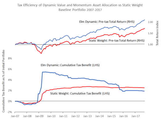
The simulation of our dynamic asset allocation approach was calculated by running our current tax-aware rebalancing algorithm over the historical period 2007-2017, but it does not include the further potential benefit of doing tax-aware “harvest” transactions at times other than on our 40-day rebalancing cycle. For the static-weight portfolio, the simulation assumes that we rebalance the portfolio back to the Baseline weights every 40 days in a tax-aware manner, also without any extra “harvest” transactions.
The chart shows that not only did Elm’s dynamic asset allocation approach provide a significantly higher pre-tax total return over the period, 110.5% versus 72.2%, but also until the end of 2015 it achieved this with greater tax efficiency too. By the end of the 11-year period, the total tax benefit delivered by our dynamic strategy falls just slightly below the net tax benefit enjoyed by the static-weight strategy, which is partly a result of the higher return of the dynamic versus static strategy during the period. The salient feature of the cumulative tax benefit of our dynamic strategy occurs in the period of late 2008 and early 2009 during the bottom of the market when our rebalancing strategy realized substantial short-term and long-term capital losses, which resulted in a long-lasting cumulative tax benefit of about 2%, or roughly 0.2% per annum amortized over the full 11-year period.
In sum, and keeping in mind the usual caveats about the past not necessarily being indicative of the future, this historical backtest does not contradict the proposition that Elm’s dynamic asset allocation strategy can deliver tax-efficiency comparable to that of a static, buy-and-hold style approach.
- Victor is the Founder and CIO of Elm Partners, and James is Elm’s CEO. Past returns are not indicative of future performance. This not is not an offer or solicitation to invest.
- And far more tax efficient than most hedge fund and other alternative investments, as discussed here.
- Half of our SMA investors who have been with us for more than six months have added to their SMA portfolios at least once. Additions tend to improve tax efficiency of returns.
- There are many other limitations to the usefulness of our example, such as the short period of time covered, the relatively benign market environment over that period, and the recognition that tax rates and law will change over time in ways that are impossible to predict.
- See here for some of the salient differences between an investment in our Fund compared to an investment in an SMA managed by us at Fidelity.
- Please see our note “What’s Past is Not Prologue” for more on the limits of historical data in investing.
- You can find our latest Baseline weights in the second table in our latest investor report here.
- This is roughly in-line with an expectation of deferring capital gains for about 20 years with an equity nominal return of about 7%.
- The annualized standard deviation of monthly pre-tax returns of the Elm Fund was 6.0% compared to 6.9% for the static Baseline portfolio over period.
- Some of the difference in blended tax rate comes from the short-term capital losses that were generated, which we assume investors can make use of to offset short-term capital gains elsewhere in their investment portfolio. Even without that benefit, our dynamic approach still achieved a slightly lower blended tax rate than the naive static weight approach.
We also note that the static approach could have achieved a lower blended tax rate if we had applied some of the same tax aware portfolio management strategies, but our purpose here was to illustrate the potential benefits of all that we can bring to bear in delivering tax efficient returns versus. a “vanilla” static-weight investment approach.
- Our Delaware fund structure also benefits, in a rising market, from new investors coming in to the fund, allowing us to buy new higher basis tax lots, and investors redeeming and taking capital gains allocations with them.
- With short-term gains weighted significantly more heavily than long-term gains. We discuss how tax considerations impact portfolio rebalancing in more detail in this note here.
- See here for more on Ben’s maxim, and here for a more general discussion of tax efficiency in long-term equity investing versus alternative investments.