By James White, Jeff Rosenbluth and Victor Haghani ¹

Thank you to the 702 people who read and interacted with our note exploring when past returns are indicative of future returns. We received so much thought-provoking feedback that we decided a follow-up note was in order.

We started by asking readers to guess how many flips they’d want to see in order to be able to discern, with 95% confidence, a fair coin from a coin biased 60% to land on heads.²

Below is a histogram of the guesses.

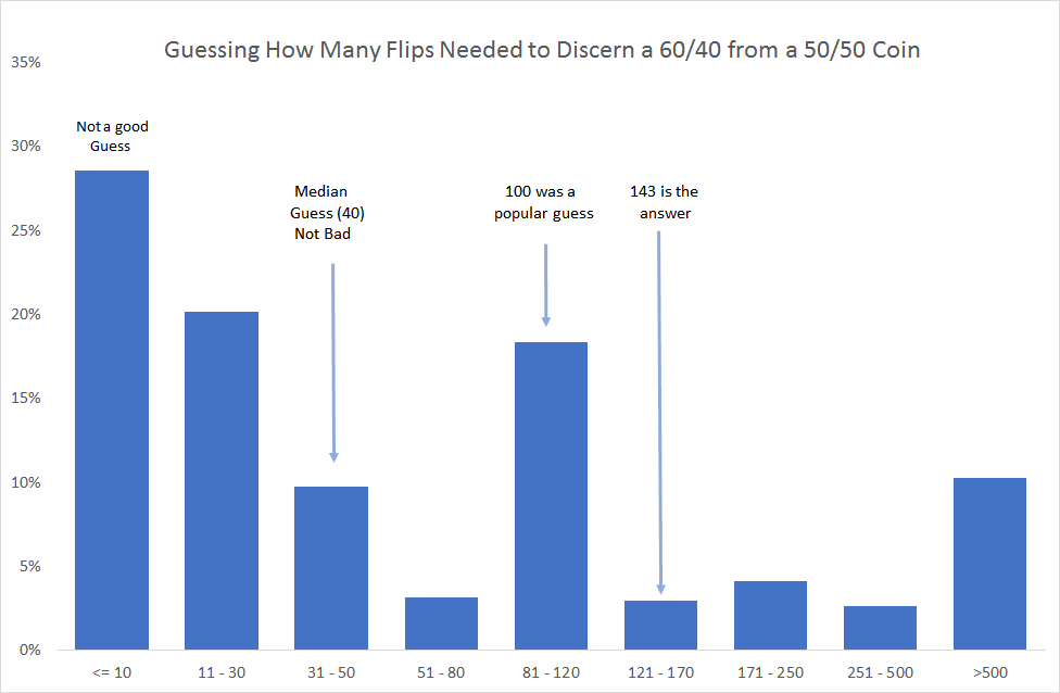
The median guess was 40 flips. While lower than the full-credit answer of 143, it does show that our readers appreciate it takes a really long time to identify an investment with this kind of risk/reward simply by track record. In Appendix I, we include the calculation used to arrive at 143.³. Our readers are a pretty mathematical bunch, and we’re sure that if they took their time to calculate an answer, rather than giving a quick guess as we requested, most would have come close to the correct answer. But the point of the exercise was to illustrate how when we are thinking fast, we tend to put too much weight on small samples: a full 30% of respondents, the single largest bucket, thought 10 flips or less was sufficient. This built-in tendency to overweight small samples can easily lead us to ignore the dictum that ‘past performance is not indicative of future results.’

Our readers generally agreed that a 60/40 coin would represent an attractive investment opportunity. At a rate of one flip per year, this would equate to an investment with a Sharpe Ratio of 0.2, roughly comparable to most broad public markets.⁴ In fact, a few suggested that 95% was too high a confidence test given the attractiveness of the opportunity. They remarked that they’d be happy to invest half their money on each coin, and not worry about figuring out which was which. This comment highlights the fact that in the two-coin problem we presented, you’ve got a 50% chance of picking the right coin without learning anything through flipping them. However, if we make the problem more realistic by asking how many flips are needed to discern a 60/40 biased coin from 3 fair coins, the number of flips required jumps to 220 (see Appendix I). So even if we had a lower confidence test but with more potential coins, as would be likely in the real world, it still takes a long time to figure out which is the good coin.

Perhaps the most thought-provoking suggestion arising from our original note came from our friend Andy Morton. He proposed a more realistic setup of the problem wherein you can invest in 100 active fund managers, but only 15% are expected to generate a post-fee return of 1% a year in excess of their benchmark, while the other 85% are expected to lose 1% a year vs. their benchmark after expenses. We’ll assume that each has an annual risk vs. the benchmark of 10%, which makes the outperformance of the good funds vs. the bad funds similar in Sharpe Ratio to a 60/40 coin vs. a fair coin. If anything, this may be optimistic given S&P Dow Jones reports that only 1 in 10 active managers outperformed their benchmarks over relatively short horizons, while with our assumptions, just under 50% of funds would outperform their benchmark each year.⁵

Let’s explore the ramifications of ‘chasing’ returns with this setup. You start off by putting 1% of your portfolio into each fund, because you don’t yet have data to tell them apart. Your starting expected return is -0.7% p.a. versus the benchmark (85% * -1% + 15% * 1% ). Each year you move more of your portfolio to the funds that have been doing well, using a Bayesian update of the probability of each fund being one of the good ones, and that helps your expected return improve from the starting point (see Appendix II for more detail). Alas, even by the end of 5 years – a reasonable ‘lookback’ window for real-world fund evaluation – the expected return versus the benchmark on your portfolio will still be -0.66%. Extending out to 10 years doesn’t help much either – you only improve to -0.6% expected return.⁶

It’s generally believed that Warren Buffett-like investors are very rare – much rarer than 1 in 1,000 – but regardless let’s say all 15 of our ‘good’ fund managers are like Buffet and produce an excess Sharpe Ratio of 0.45 (roughly Berkshire’s Sharpe Ratio of excess returns versus the S&P 500 since 1980). In this case, after 5 years we’d still only be breaking even across the whole portfolio, and would only have about 50% of our capital allocated to the 15 Warren Buffetts! We can clearly see that in the real world, where Buffetts are much rarer, 5 to 10 years of track record just doesn’t tell us that much when dealing with a portfolio composed mostly of mere mortals.

As we discussed in our note from six months ago, ‘What I learned from my daughter (about investing)’, our attempt to build a portfolio of rare investment gems – a clutch of young Buffetts – also has to contend with the drag of the false positive. Even if we can identify a good from a not-so-good investment with 90% accuracy, if the good ones represent just 5% of the possible investments, the best we can expect is a portfolio comprised of 32% good ones and 68% not-so-good ones. The cognitive bias that makes it hard to see this result is called base-rate bias.

In the real world, any kind of return-chasing strategy will also face additional headwinds, amongst them the fact that when an investment strategy was truly extraordinary in the past, its very discovery will diminish future performance (or even make future returns negative), as more capital is drawn towards it. This may be the the prime reason why investor returns (i.e. dollar-weighted returns) tend to be significantly below fund returns (i.e. time-weighted returns).⁷ This doesn’t happen with coin flips.

Another comment worth sharing, from the marketing capo of a well-established hedge fund group, was, ‘I don’t know anyone who would look at a fund investment without looking at the past track record.’ We think the reason for this, and perhaps the central problem with investing in active fund managers, is that there is virtually no other way to develop a forward-looking expectation other than to look at the past track record. Unfortunately, as we’ve illustrated with our two-coin example, there is very limited statistical power in the typical historical return dataset which is often limited to 3-5 years due to issues around manager turnover.

Perhaps when a fund picker says, ‘We only will look at funds that have at least a 3-year track record,’ he is thinking that if he observes the funds on a weekly basis, that gives him a lot more data points to draw upon to reach a good level of confidence. Unfortunately, it doesn’t help because when we observe the managers on a more frequent basis, it’s requiring us to discern a coin that is closer to 50/50, which takes exactly the extra flips you get by sampling more frequently. Bob Merton pointed this out in a 1980 paper titled, ‘On Estimating the Expected Return on the Market,’ …nothing is gained in terms of accuracy of the expected return estimate by choosing finer observation intervals for the returns.’ ⁸

One more remark we think worth sharing was, ‘An investment in a fund is always about the manager.’ That at least recognizes the limited value of past returns, especially in isolation and over typical, relatively short horizons. The problem is it’s very hard to separate our qualitative evaluation of a manager’s character from our knowledge of their track record – most managers with an apparently sterling, but often short-term, track record also present as highly confident and competent people, in a way which might not be the case with a different frame.

Once you accept the very low discriminating power of past returns in most practical investing contexts, what are you to do? Of course, you’ll want to look at all the information at your disposal regarding any investment, and track record should be part of the due diligence of any investment. If it’s particularly long and distinguished, it might have some impact on your forecast, when used together with other factors. It just shouldn’t be the primary or isolated driver of your return forecast. And if you’re ever unsure whether you’re being unduly influenced by a good track record over a normal (relatively short) time horizon, ask yourself whether you’d still make the investment if the return had been half as bad as it was good. If you answer yes, you’re probably giving about the right weight to track record in your decision process.

All this discussion on the low value of historical returns in most investment contexts may leave you feeling either depressed or liberated, depending on your perspective and occupation. If you’re an investor, it’s really not so bad: just stick to investments where you don’t need to rely on the track record to make your decision. That leaves almost all of the direct, cost-efficient, investible universe open to you– bonds, equities, real estate and any strategy where you can produce a reasonable forward-looking return estimate without relying on past returns.

---

Appendix I: Flipping a biased coin and one or more fair coins

We would like to calculate how many flips of 2 coins, one biased and one fair we need to be 95% confident that the coin with more heads is the biased one. Above, we assumed that the biased coin has probability of heads of 0.6, here we will be a bit more general and represent this probability by p . Since each coin has a binomial distributions and the coins are assumed independent, the joint probability mass function of the two coins after n flips is the product of two binomial probability mass functions. Denote by Q(n,k,j) the probability of k heads for the biased coin and j heads for the fair coin after n flips, thus

  Q(k,j,n) = (nk)  p^k  (1 – p)^{n – k}  (nj)12^j12^{n – j}

This allows us to calculate the probability that the coin with more heads is biased as

  1 2ⁿ Σ j < k k ≤ n ( n k ) ( n j )  p^k  (1 – p)^{n – k}

Choosing n to be 143 and p = 0.6 , we obtain 95.01%.

If we have more than one fair coin, the analysis is very similar. We calculate the joint probability mass function for the biased coin and the fair coins simply by multiplying together the individual probability mass functions. Then we sum over all of the cases where the biased coin has more heads than the maximum heads of any fair coin. All though this is a closed form solution, the summation has way too many terms to handle by hand. Therefore, we enlist the aid of a computer to calculate it.

---

Appendix II: Bayesian Capital Allocation for 100 Funds

In our 100 fund example from above, we used a ‘return-chasing’ capital-allocation rule based on Bayesian learning, and here we explain the logic behind that in more detail.

Bayes’ Theorem (sometimes also called Bayes’ Rule) provides a powerful tool for updating our beliefs about the world as new information is received. In the 100 funds example, for each fund we would have a level of belief about whether that fund is in the Good group or the Bad group. Before we have any data, our belief that a given fund is good would be at 15% for each fund. As we have incremental data about fund performance, we can use Bayes Theorem to update our level of belief for each fund, in a way that’s rigorous and consistent with the information-value contained by the new data. Specifically, we update our level of belief by the relative likelihood of seeing the new data if our hypothesis is true versus if it’s false. To give a simple example: if we get new data in, and that particular data is no more likely when our hypothesis is true versus when it’s false, then our level of belief stays the same. On the other hand, if we get in new data and that data is highly likely if our hypothesis is true, but highly unlikely if it’s false, then our level of belief will go up substantially.

Bayes’ Theorem: For a hypothesis H with prior probability P(H) and new data D with P(D) ≠ 0 then,

  P(H|D) = P(D|H)P(H) P(D)

Using the mechanics of Bayes’ Theorem and assuming that capital is allocated proportionally to our level of belief that a fund is in the Good group, we can derive a closed-form solution for the mathematical expectation of capital that would be allocated to the Good funds at each point in time as more fund data becomes known. We can also see in closed form the mathematical expectation of the updated probability that a Good fund is good and a Bad Fund is bad, at each point in time:

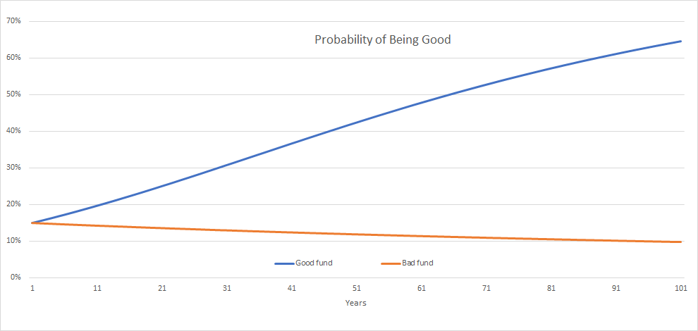
As we can see from the above chart, even with this fairly sophisticated update strategy, relatively short periods of time don’t meaningfully impact our probability estimate that a Good fund is Good, or that a Bad fund is Bad.

---

1. James is Elm Partner’s CEO, and Victor is the Founder and CIO. Past returns are not indicative of future performance. This not is not an offer or solicitation to invest.
   
2. Example inspired by: ‘Good and bad properties of the Kelly criterion,’ MacLean, Thorp, Ziemba, 2010, page 8.
   
3. Another version of the problem, posed and solved by Costas Kaplanis, lets the observer stop the flipping whenever desired. In this version of the problem, the solution involves using Bayes’ Theorem to update the probabilities regarding the identities of each coin. The result is that you usually need significantly less than 143 flips to be 95% confident you’ve identified the correct coin, but there is still a significant probability that you will need well in excess of 143 to get to that level of confidence. Stay tuned for more from Costas on this topic.
   
4. We did have some respondents who suggested that they only invest in opportunities with a Sharpe Ratio of 1 or higher. In our experience, investments that appear to have such high Sharpe Ratios are closed to outsiders, implicitly bear significant, hidden negative tail risk, are ephemeral or, infrequently, are fraudulent. For a more academic treatment, see Harvey, Liu, Zhu, ‘…and the Cross-Section of Expected Returns’, (2015), on SSRN.
   
5. See SPIVA Persistence Scorecard here for S&P Dow Jones report.
   
6. We can make the example more realistic by introducing some mean-reversion into the picture in order to capture the effect that when an investment strategy truly was extraordinary in the past, its very discovery will tend to diminish future performance (or even make future returns negative), as more capital is drawn towards it.
   This doesn’t happen with coin flips. The result is that a moderate amount of this effect means that even if the good managers are generating 4% more return than the not-so-good managers, even after 50 years the expected return of your portfolio still won’t be positive.
   To give this result some context, this amount of excess return is similar in risk-adjusted terms to Warren Buffett’s past 40 year track record relative to the S&P 500. The amount of mean-reversion we introduced is such that each fund is expected over the coming year to make back or give up 20% of the return it lost or made relative to the benchmark and to its underlying expected return over the past five years.
   So, if a fund outperformed by 10% over the past five years, it would be expected to do 2% worse than its normal expected return over the next year. Of course, a strategy set up to explicitly take advantage of the mean reversion would do better, but that is the topic for another note.
   
7. See our Elm paper on return-chasing here. Also, see Morningstar’s ‘Mind the Gap’ notes and Dalbar’s annual investor behaviour reports.
   
8. Merton, Robert, C., On Estimating the Expected Return on the Market: An Exploratory Investigation, Journal of Financial Economics 8 (1980) 323-361. See Appendix 1, pages 355-357. To see why you can’t get around this inconvenient truth, note that in continuous time, the number of years of observation, using the annual Sharpe Ratio (SR ) as an input is 2 * (1.645 / SR)² , where 1.645 is the 95% cumulative probability level in a Normal distribution. If we sample more frequently, f times per year, the required number of periods goes to 2 * (1.645 / (SR√f))² = 2f * (1.645 / SR)² .
   So, we’ll need to observe f times as many periods as when we look annually, which is exactly how many more periods we get to observe by breaking the year into f intervals. Note this exact result depends on a strong assumption about the distribution returns are being drawn from.