April 16, 2020
Investment Theory
George Costanza At It Again: The Leveraged ETF Episode
By Victor Haghani and James White 1
Sometime in late 2018…
George: How about this stock market? Down 14% in three months. It’s killing me. Day after day and all I see are big red numbers next to every single one of my investments. Everything I buy goes straight down – I can’t take it!
Kramer: Ooooooweee, buying stocks is no good.
George: No good?
Kramer: Here’s a can’t-lose strategy for you: invest half your money in SPXL and the other half in SPXS.
George: I never heard of these stocks before – what are they?
Kramer: They’re not stocks, they’re ETFs – Exchange Traded Funds, and they’re TURRRRBO-charged! SPXL is a 3x leveraged long S&P 500 ETF and SPXS is a 3x leveraged short S&P 500 ETF. There’s no limit to how much they can go up, and you can’t lose more than you put into them. One or the other is gonna make you rich. Kaching!
George: It’s gotta be better than what I’m doing now. What could possibly go wrong?
15 Months Later…
George: KRAMER!! What’d you do to me?!!? I should never have listened to you.
Kramer: What are you talking about? What’s the problem?
George: It’s those two leveraged ETFs you told me about. The stock market is up 6% since our little chat, but SPXL and SPXS are both down big – one is down 20% and the other one is down almost 50%!
Kramer: Hmmm…doesn’t seem possible. I’ve got another idea: have you ever thought about doing the opposite of whatever you think is a good idea?
George: I tried that already, and I’d rather not talk about it.2
Leveraged ETF Returns: Not What George Was Expecting
George’s surprise at losing on both SPXL and SPXS is understandable; they sound like direct opposites of each other. Given the 3x leverage and the stock market up 6%, he probably expected SPXL to be up about 18% and SPXS to be down about 18%. Instead both under-performed the ‘expected’ result by over 30%. The ETFs were not poorly managed, and the relatively high fees (about 1%) can’t come close to explaining the performance gap. In understanding what’s going on with these ETFs, we’ll uncover an important lesson relevant to all investing, about how your choice of investment size can be more important than your choice of investment.
These highly leveraged long and short ETFs provide a perfect illustration of how overly-aggressive investment sizing can turn a good trade into a losing one. An investor who borrows money to take a leveraged position in an asset will need to keep trading the asset in order to maintain a constant level of leverage as the asset price fluctuates. For example, 3x leveraged ETFs are structured and labeled as being constantly 3x leveraged through time, on a daily basis. For a 3x long ETF, that means the ETF needs to buy every day asset prices go up, and sell when they go down. This creates a nasty surprise: if the S&P 500 starts at 2500, goes up to 3000 one day, then back to 2500, the 3x-long ETF has to buy at 3000 and then sell at 2500, locking in a loss over the two days even though the market is flat. We’ll refer to this locked-in loss that comes from trading to maintain constant leverage as ‘volatility drag.’3 Over any given day, the 3x leveraged ETF return is equal to 3x the daily return – but over multiple days, because of this daily trading, the 3x leveraged return will be lower by an amount that depends on how volatile the market has been.4
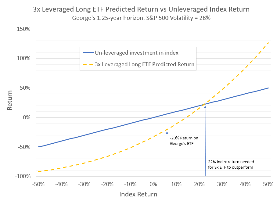
High leverage combined with high realized volatility has a powerfully negative impact on returns, enough to explain George’s realized return of -20% for SPXL and -50% for SPXS relative to the market return of +6%.5 In the chart below, we show how George’s 3x-leveraged long ETF would have done over a range of returns for the S&P 500, given the 28% realized volatility of the stock market over his holding period.6 For SPXL to have outperformed an unleveraged investment, the market needed to go up by more than 22% to overcome the leverage-induced volatility drag.
Market Impact of Leveraged ETFs: 1987 Portfolio Insurance Redux?
Even though George hadn’t heard about these leveraged ETFs, they’ve been around since 2006 – and they’ve grown to be more than a side-show in the marketplace. According to Lara Crigger’s research at ETF.com, leveraged ETFs had assets of close to $40 billion at the end of March 2020,7 and that’s just tallying up the US-listed structures that are publicly registered – there’s likely considerably more in privately-structured products and non-US vehicles.
To gauge the potential market impact of these leveraged long and short ETFs, let’s take a closer look at what trades SPXL and SPXS would have to execute after a 10% market rise:
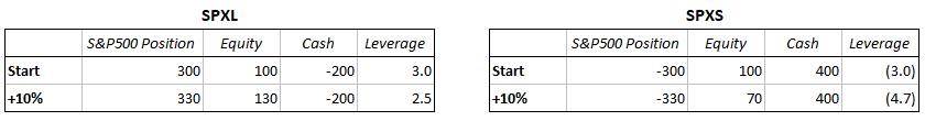
We can see that after this 10% market rise, SPXL is now under-levered and SPXS is over-levered. To return to 3x-long and 3x-short, both ETFs need to buy more S&P 500. SPXL needs to buy $60 of the S&P 500 and SPXS needs to buy $120. If the market falls instead, the numbers are the same but the ETFs will need to sell. As you can imagine, the turnover within these levered funds can be enormous; for a 3x leveraged-long ETF assuming 1% daily moves (16% annualized), annual turnover would be 1500%, and 3000% for a 3x leveraged-short ETF.
In terms of the potential market impact of the trades these ETFs need to do each day, we estimate that the managers of these public leveraged ETFs need to buy or sell about $10 billion of equities when the stock market goes up or down by 5%, and most of that trading has to happen near the closing bell each day. Of course, many market participants are aware of these, and other similarly predictable flows coming from options-hedging and leveraged investment strategies such as Risk Parity and volatility targeting funds. In trying to profit from these anticipated flows, opportunists smooth them out and make them harder to pinpoint, but their impact doesn’t completely disappear.8
Sizing Your Stock Market Exposure for the Long-Term
As you know from our other research notes, we think choosing your equity allocation should be a forward-looking exercise, driven by your assessment of future return and risk, and your own circumstances and personal level of risk aversion. That said, it’s still interesting and instructive to take a look back sometimes, and we’re going to take a look at how different levels of stock market exposure – including leveraged – would have performed over the long-term.
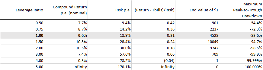
From 1927 to the end of March 20209, the annualized total return on the S&P 500 was 9.6%, which would have turned a $1mm investment into $4.5 billion today – not too shabby. Average stock market volatility was just under 19%, and T-Bills returned 3.7% p.a. If you were around in 1927 and had a crystal ball, wouldn’t you have been tempted to invest in equities on margin and really make a killing for your lucky descendants? After all, if investing 100% of your savings in equities for the long-term was sure to be great, why not invest 200% or 300% of your savings?
The table below works through this thought experiment, showing how things would have turned out for an equity investor taking on different amounts of leverage over those nearly 100 years.10 Notice that 1.5x leverage leaves you with the most money at the end, but at some point you’d have experienced a drawdown of 95%. Above 1.5x leverage, return goes down and risk goes up, driven by the volatility drag we’ve been discussing. At 4x leverage, after suffering more than a 99.99% drawdown, you’d eventually only be left with the $1 you started with (just $0.09 inflation-adjusted), and at 5x leverage you’d have been fully wiped out on October 19th, 1987. Here’s an interesting thought-experiment: what equity exposure would you have chosen standing in 1927 with the crystal ball?11
Opposite George?
What if George followed Kramer’s advice, and did the opposite of whatever he thought was a good idea so instead of buying these two leveraged ETFs, he shorted them? As we explained in our first note about George’s investing, being short is not the opposite of being long. In fact, if we assume that an investor shorting either of George’s ETFs wants to keep the value of her short equal to her capital in the trade (including unrealized losses or gains along the way), then being short the 3x leveraged long ETF looks exactly the same as being long the 3x leveraged short ETF, and vice versa.
The closest thing to achieving the opposite of the leveraged ETFs’ volatility drag would be to invest in a balanced portfolio, such as 50% equities and 50% T-bills. Maintaining the 50% / 50% weight over time would require buying equities when they go down and selling when they go up, creating a volatility ‘lift’ instead of a ‘drag’ from the portfolio rebalancing. Unfortunately, this lift is naturally limited in scale – you can create as much drag as you want by using large leverage, but you can only get the maximum lift by maintaining a position size at 50% of total capital.
Conclusion
A big problem with holding these leveraged long and short ETFs for more than one day is that most investors are likely to think they are making a decision based on a view of where the market is going: up or down. As we’ve explained though, that’s not typically what they’re getting.12 Rather, the return on a leveraged long or short ETF held over time will incur a drag that increases dramatically with both leverage and realized volatility. As George’s experience attests, the investor can have the right call on market direction while the investment outcome is overwhelmed by the impact of high realized volatility.
The exchange between George and Kramer is fictional, but the disappointing returns on George’s two leveraged ETFs are sadly quite real. The lesson from George’s misadventure isn’t only for those thinking about investing in highly leveraged ETFs. For all investments, as position size increases, there’s a point beyond which you’ll be more likely to wind up with losses than with gains, and further still, an amount of exposure at which you’ll be almost assured of losing all your money. Much of the art of investment sizing lies in appreciating and optimizing where on the curve is right for you.
Further Reading and References:
- “Report of the Presidential Task Force on Market Mechanisms.” The Brady Commission, January 1988.
- Cheng, Minder and Ananth Madhavan. “Dynamics of Leveraged and Inverse ETFs.” Q-Group, 2009.
- ETF Research Collection. Professor Tim Leung, Columbia University.
ETF Database:
ETF.com
- Crigger, Lara. Leveraged ETF Closues Piling Up
- Crigger, Lara. Why These Leveraged Energy ETPs Tanked
- Crigger, Lara. Don’t Buy and Hold Leveraged ETFs
- Crigger, Lara. The Truth About Leveraged ETF Returns
- UWT ETF Profile Page (via FactSet)
- DWT ETF Profile Page (via FactSet)
- This not is not an offer or solicitation to invest, nor should this be construed in any way as tax advice. Past returns are not indicative of future performance.
Thank you for the very helpful comments from our friends Antti Ilmanen, Chi-fu Huang, David Modest, Jeffrey Rosenbluth, Josh Haghani, Lance McGray,Lara Crigger, Mark Haghani, Richard Dewey and Samir Bouaoudia, and a special thanks to Larry Bernstein for bringing these ETFs and their perplexing performance to our attention.
- See our note If George Costanza Were a Hedge Fund Manager for more of George’s mis-adventures in investing. Inspired by Seinfeld Season 5, Episode 22, ‘The Opposite.’
- If the investor chooses not to rebalance the portfolio, the volatility drag is transformed from a relatively constant cost through time into a path-dependent, one-off risk of total wipeout, without changing the overall expected outcome.
For example, if the two ETFs George had invested in started at 3x leverage and then did no rebalancing, the result would have been that SPXL would have returned about +12%, but SPXL would have lost 100% in mid-February 2020, when the S&P 500 had gained over 33.3% since the start of George’s investment. So, with no rebalancing, George’s combined ETF investment would have lost 44%, rather than the loss of 35% on the daily rebalanced ETFs we’re discussing in this note. Of course, this was just one path, but it’s a good illustration of how the rebalancing frequency introduces path dependency.
- Here’s a formula which explains the poor performance of George’s ETFs:Retf = L * R̂index – (L * σindex)2 / 2where Retf = ETF daily return which can then be compounded up to get a return for the period desired,
L = leverage ratio, positive if long and negative if short,
R̂index = the average daily return of the index, and
σindex = the standard deviation of the daily returns of the index. For simplicity, we assume that the risk-free rate is zero. The formula assumes the index follows a geometric Brownian motion. - To explain George’s return on the 3x Leveraged Long and short ETF, we need the following information: average daily return on index= 0.0325%, daily stdev on index = 1.74%, daily avg T-bill rate = 0.0059%, 314 days in period. Plugging these into the formula in footnote 4 we get expected losses of 15.4% and 47.5%, compared to actual losses of 20% and 50%, on the 3x leveraged long and short ETFs respectively. The balance of the losses is mostly explained by the 1.06% pa fees on both ETFs and the cost of leverage incurred in the ETFs being worse than the T-bill rate we used.
- We assume the ETF finances its leveraged position at 1% above the average T-bill rate, and that the ETF charges a fee of 1% p.a.
- Split about 50/50 between 2x and 3x leveraged ETFs, 60/40 between long vs short, and about 75% in equities.
- It’s hard to know the impact of flows of this size. Although it’s a datapoint from a long time ago (when the US stock market was about 10% of its current size) the Brady Commission’s report on the October 19, 1987 stock market crash estimated that about $6 billion of selling by Portfolio Insurance programs over the course of the whole day was primarily responsible for turning a bad day into the worst day ever, -22.5% for the US stock market.
- We chose that period as it’s the longest for which we can easily find daily S&P 500 data.
- The table assumes daily rebalancing, no transactions costs, no fees, no impact, borrowing at 3 month T-bill rates +1%.
- Robert C. Merton, in his 1969 paper Lifetime Portfolio Selection Under Uncertainty, suggested a simple formula, subject to a stylized set of assumptions, for determining how much equity exposure one should optimally take based on the expected excess return of equities over the return of the risk-free asset, the risk of equities and the degree of personal risk aversion of the investor.
For an investor whose crystal ball gave a precise estimate of the expected return and risk of the equity market over the 1927-2020 period that matched the realized market experience, and who had a level of risk aversion in line with investors we surveyed in our 2018 study,(coefficient of risk aversion = 2.5) the optimal equity allocation would be about 85%.
- The few leveraged ETF prospectuses we’ve reviewed explain this as well.