By Victor Haghani and James White ¹

Encouraged by some of our investors, we are introducing a new fund for non-US investors, the Elm Partners All Equity Portfolio (EPAEP). EPAEP will have a Baseline of 100% Global Equities, in contrast to our current Global Balanced Fund which has a Baseline of 65% Global Equities, 5% Commodities, and 30% Global Fixed Income.

The Fund will be managed algorithmically with a dynamic asset allocation driven by valuation and momentum, in line with the Active Index Investing® approach we’ve applied since 2012 to our Global Balanced portfolios. EPAEP will use low cost ETFs, will charge our standard 0.12% per annum management fee and will maintain our usual focus on cost and tax efficiency. The Fund will be long-only, un-levered, and will always have a target of being fully invested in global equities. This note describes details of the asset allocation methodology, implementation and historical return simulation. Please feel free to email info@elmwealth.com or set up a call with us if you’d like to learn more or request a Prospectus.

Target Investor Group

The All-Equity Fund is designed for non-US investors who want Elm’s global diversification and value-and-momentum approach to equities, but who want a relatively constant amount of equity exposure or want to manage their cash and fixed-income assets on their own.

In contrast, Elm’s Global Balanced Fund is designed for investors who want Elm to dynamically manage their exposure to equities versus fixed-income, with a balanced 70%/30% Baseline Asset Allocation as the starting point. This may be suitable for investors who want Elm to manage a meaningful fraction of their liquid wealth, who want to be more hands-off with their asset allocation, and who want an investment program with a risk level that varies through time as a function of the attractiveness of available investments.

Investors can also invest in both the Global Balanced and All-Equity Funds to achieve a Baseline risk level in between that of the two funds. This may be suitable for investors who want the dynamic risk level of a Balanced program, but who have a tolerance for a higher level of variability and expected return. With the normal caveats about past returns not being predictive of the future, simulated historical returns for the All-Equity program over the past roughly 40 years had about 50% more variability and 20% higher real returns than did the Global Balanced strategy, as described more fully in the Historical Simulation section below.

Background

Elm’s Active Index Investing® attempts to combine the best features of active investing and index investing to deliver superior long-term risk-adjusted returns. We do not follow the market-cap-weighting regimes of MSCI or FTSE, but rather we systematically construct our own Baseline Asset Allocations which we feel are more representative, diversified and risk/return efficient. We then add a dynamic overlay to our Baseline, following the principle that allocations should be proportional to forward-looking expected real returns, and drawing on value and momentum as the two primary indicators of expected returns. Allocating proportionally to expected real return has deep roots in Samuelson and Merton’s work on Decision-Making Under Uncertainty starting in the early 1960s,² and commonly used applications such as the Kelly Criterion. In turn, the value and momentum perspective was popularized by Asness, Moskowitz and Pedersen in their seminal “Value and Momentum Everywhere” paper, and by our own research including “A Case Study for Using Value and Momentum at the Asset Class Level,” in the Journal of Portfolio Management, which traced this market phenomenon back to 1925.³

We use a value-and-momentum-driven approach to asset allocation because we believe that:

• Simple valuation metrics like the Cyclically-Adjusted Earnings Yield of a broad equity market are robust predictors of the market’s long-term expected real return,
• Momentum is a good medium-term predictor because investors have a tendency to extrapolate future market returns from recent historical samples, which results in trends generated by “return chasing” behavior, and
• Value and momentum signals often yield offsetting recommendations, which makes them more effective when used together than individually.

We are attracted to broadly diversified, rules-based investing which index products tend to facilitate, and to the cost and tax efficiency of index products. One of our core principles is to focus on costs, and you can see our note here on why we think reducing costs is even more important than meets the eye to maximizing investor risk-adjusted returns.

Methodology

We start by constructing an All-Equity Baseline portfolio intended to be more representative of the Global Market Portfolio than the adjusted-market-capitalization indexes of MSCI and FTSE, with a moderate “home bias” preference for OECD non-US investors. The process is the same as applied to constructing our Global Balanced Baseline, except in the All-Equity Baseline we put a 0% weight on fixed income assets.

The next step is to determine, at each portfolio rebalancing date, desired deviations from the Baseline weight of each asset bucket using a combination of a valuation metric and a momentum indicator. This is also done largely in the same way as we do for our Global Balanced program, with several modifications to fit the context of an All-Equity portfolio. Most significantly, we normalize the target weights so that they always sum to 100%, and we also impose a constraint that no bucket’s target weight can be more than twice its Baseline weight.⁴ We measure momentum for each asset class relative to the return of the Baseline⁵ and we’ve reduced the intensity of the value signal to counter the amplification which can result from the target weight normalization process.⁶

The table below shows the Baseline weights and the desired targets as of March 31, 2020.

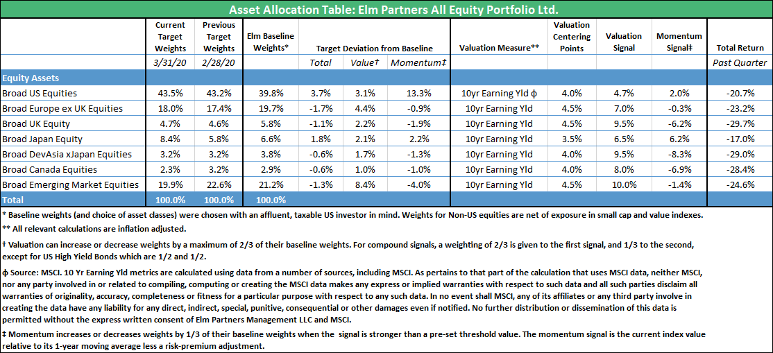
You can find more detail on our Baseline construction and value and momentum overlay here.

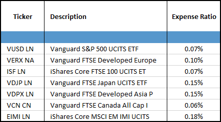
Implementation

We will manage EPAEP using Elm’s proprietary Ulmus portfolio management system, and will rebalance the portfolio twice monthly. We expect portfolios to have weighted average expense ratios (excluding Elm’s 0.12% pa management fee) in the range of 0.10 to 0.12% per annum, and over time we expect ETF fees to decrease even further. The table below shows a sample of the instruments we intend to use to build the Fund’s portfolio, though many more instruments are in our database for consideration and possible use.

The Fund has monthly liquidity, on the last business day of each month with at least 3 business days notice.

Historical Simulation

As usual, we stress that historical data on its own is not sufficient to establish that an investment strategy such as the one outlined in this note is a good one. We are firm believers that past returns are not indicative of future performance. However, history can lead us to conclude that a strategy is poor, and it is with that perspective that we look to the past.

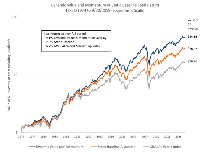
The chart below shows a simulated back-test from December 31, 1974⁷ to September 30, 2018. Our All-Equity program’s dynamic value and momentum overlay added 1.3% pa of extra return with no material increase in volatility, sampled monthly, versus the returns of a static weight All-Equity Baseline portfolio. This is in line with what we would have expected given that the value and momentum overlay applied to the Global Balanced Baseline increased returns by 2.7% a year with no material increase in volatility over roughly the same historical period, as we reported in our 2016 Journal of Portfolio Management paper. This makes sense as the Global Balanced portfolio has more flexibility to vary its asset allocation compared to the All-Equity program.

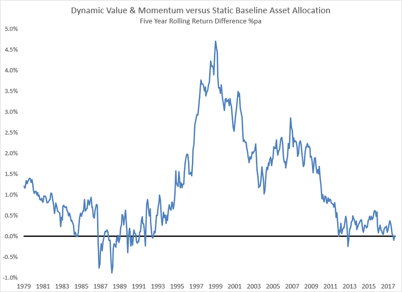
The variability of the difference in returns between the dynamic and static All-Equity portfolios was 1.9% pa, sampled monthly, suggesting a Sharpe Ratio for the dynamic versus static strategy of 0.7 over the full period. This is consistent with the finding that the value and momentum overlay resulted in outperformance 60% of the time to a monthly horizon. However, as we’d expect, to a longer-term horizon of five years the outperformance was more consistent, occurring in 97% of 466 rolling five-year periods evaluated at the end of each month. This is shown in the chart below.

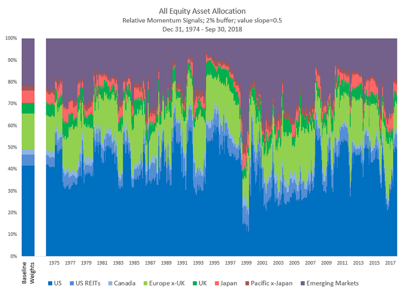
The final chart shows the simulated historical desired asset allocation of the dynamic value and momentum asset allocation. Portfolio turnover over the period averaged 60% per annum. In practice we expect lower turnover, as rebalancing would be every 40 days rather than monthly and we generally do not rebalance every bucket back to its exact desired weight.

Finally…

Please be in touch with any questions or suggestions. You can request a short presentation and fund Prospectus here.

---

Note:

This is not an offering document. Past returns not indicative of future returns. The value of an investment and the income from it can fall as well as rise and you may not get back the amount originally invested.

---

Further Reading and References:

• Asness, C.S., T. J. Moskowitz, and L. Pedersen. “Value and Momentum Everywhere,” Journal of Finance, Vol. 68, No. 3 (2013), pp. 929-986.
• Blitz, D., and P. van Vliet. “Global Tactical Cross-Asset Allocation: Applying Value and Momentum Across Asset Classes,” The Journal of Portfolio Management, Vol. 35, No. 1 (2008),
  pp. 23-38.
• Campbell, J., and R. Shiller. “The Dividend-Price ratio and Expectations of Future Dividends and Discount Factors.” Review of Financial Studies, 1 (1988), pp. 195-228.
• Cochrane, J. “The Dog That Did Not Bark: A Defense of Return Predictability.” Review of Financial Studies, Vol. 21, No. 4 (2008), pp. 1533-1575.
• De Grauwe, P., and M. Grimaldi. “Bubbling and Crashing Exchange Rates.” Working Paper, CESifo (Series No. 1045), 2003.
• Dewey, R., and Haghani, V. “A Case Study for Using Value and Momentum at the Asset Class Level.” Journal of Portfolio Management, volume 42 number 3, (Spring 2016).
• Fama, E.F., and K.R. French. “Business Conditions and Expected Returns on Stocks and Bonds,” Journal of Financial Economics, 33 (1989), pp. 25-49.
• Fama, E.F., and K.R. French. “Dissecting Anomalies.” Journal of Finance, 63 (2008), p. 1653-1678.
• Ferson, W. E., and C. Harvey. “The Variation of Economic Risk Premiums.” Journal of Political Economy, Vol. 99, No. 2 (1991), pp. 385-415.
• Gnedenko, B., and I. Yelnik. “Dynamic Risk Allocation with Carry, Value and Momentum.” Working paper, ADG Capital Management LLP, 2014.
• Jegadeesh, N., and S. Titman. “Returns to Buying Winners and Selling Losers: Implications for Stock Market Efficiency.” Journal of Finance, Vol. 48, No. 1 (1993), pp. 65-91.
• Kahneman, D., and A. Tversky. “Judgment Under Uncertainty: Heuristics and Biases.” Science, Vol. 185, No. 4157 (1974), pp. 1124-1131.
• Moskowitz, T.J., Y.H. Ooi, and L.H. Pedersen. “Time Series Momentum.” Journal of Financial Economics, Vol. 104, No. 2 (2012), pp. 228-250.
• Pirrong, C. “Momentum in Futures Markets.” Working paper, University of Houston, 2005.
• Soros, G. The Alchemy of Finance. New York, NY: Simon and Schuster, 1988.
• Wang, P., and L. Kochard. “Using a Z-score Approach to Combine Value and Momentum in Tactical Asset Allocation.” Working paper, Georgetown University Investment Office, 2011.

---

1. This not is not an offer or solicitation to invest, nor should this be construed in any way as tax advice. Past returns are not indicative of future performance.
   
2. See our notes here and here for a deeper discussion of this body of work.
   
3. A working paper version of Value and Momentum Everywhere, Asness, Moskowitz and Pedersen, was in circulation from 2009 SSRN here, and presented at the 2010 AFA meeting, although the paper only appeared in the Journal of Finance in 2013.. You can find a copy of our paper here.
   
4. To normalize the target weights to 100% and impose the 2x constraint we iteratively impose the constraint and re-normalize until both the normalizing condition and the constraint are fully satisfied.
   
5. This is also consistent with the treatment of momentum signals in this early paper on implementing value and momentum in an asset allocation context: Blitz and Van Vliet, “Global Tactical Cross-Asset Allocation: Applying Value and Momentum Across Asset Classes,” Journal of Portfolio Management (2008).
   
6. We set the slope of the value signal in the All-Equity program to 0.5, in contrast to 1 in our Global Balanced programs.
   
7. Many of the historical data series we need for this analysis begin December 31, 1974, particularly the MSCI data series for regional equity market total returns and earnings.