Each of our strategies follows our rules-based asset allocation methodology, an approach we call Active Index Investing®. This note describes in detail the three main components of this approach: the construction of the Baseline portfolio and the value and momentum overlays to that Baseline portfolio which make the portfolio responsive to changing market conditions.

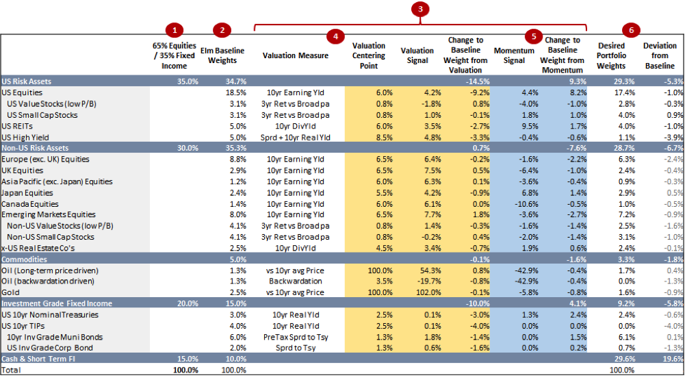
Throughout this discussion, we will use our Global Balanced Portfolio for US taxable investors as an example and refer to Table 1 below, which is a snapshot of our signals at the end of March 2015. We publish this information every month on our website and intra-month data is available on request.

Table 1: Asset Allocation Table

Risk Level

For each of our strategies, the starting point is to choose the desired level of risk in terms of an equity / fixed income portfolio. For our balanced global asset allocation for US investors, we use a 65%/35% split: 65% global market cap weighted equities, and 35% in US fixed income and money market investments. We expect this to remain constant throughout the life of the strategy.

We do not benchmark ourselves against this portfolio in the traditional sense, in that it plays no role in portfolio management decisions, but instead it can be used by investors as a potentially helpful reference point to provide a context for the targeted risk level of the portfolio and long term return expectations.

Baseline Portfolio

Based on the targeted risk level as described above, we construct our Baseline Portfolio, which is comprised of approximately 20 asset buckets (as listed in the first column of Table 1).¹ The Baseline Portfolio is not market cap weighted. It is constructed to be more balanced and diversified, with exposure to more sources of return, than the more traditional 65/35 equity/fixed income portfolio.

We believe that slavishly relying on market capitalization weights of public market equities published by providers such as MSCI and FTSE is an approach that can be improved upon. Taking account of other considerations (such as GDP, population and corporate earnings) leads to a more diversified and balanced portfolio which is more representative of all global risk assets, public and private. Such a portfolio will better approximate market cap weights in the long-term future with fairly valued markets. This approach mitigates “the tyranny of indexing” by tempering the high weights given to markets with relatively high valuations (recall that the Japanese equity market in 1989 represented 40% of a global market-cap weighted equity index).

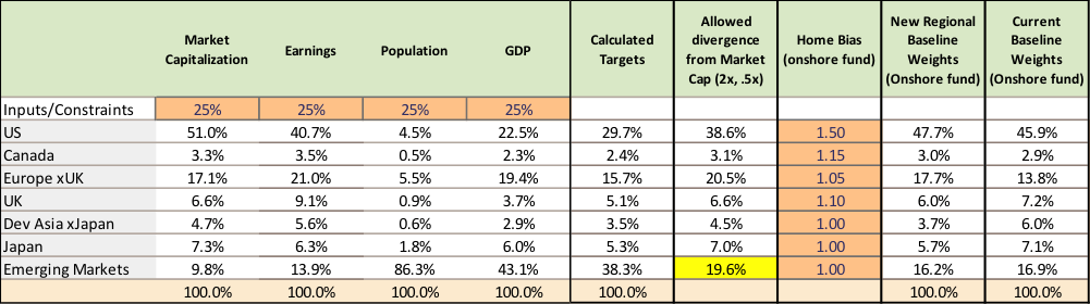
We begin by calculating the target regional weights that we will apply to our risk asset allocations. Table 2, below, illustrates our quantitative approach to determining these weights. We give equal weight to market capitalization, cyclically adjusted corporate earnings, population and GDP for each regional equity market. As developing economies (EM) represent 86% of world population and 43% of world GDP, this approach results in a desired weight of nearly 40% to EM. We feel that this would be too much of a deviation from a conventional balanced world portfolio, and so we apply a cap and a floor to all regions limiting their weights to a maximum of two times, or a minimum of one half, their market capitalization weights. These constraints are currently binding only in the case of EM, capped at 19.6%.

As this strategy is structured for US investors, we incorporate a “home bias,” reflecting the greater relevance of US equities to US investors, for example in terms of future consumption. We have set the home bias factor at 1.5 for the US, and between 1.0 and 1.15 for other regional markets.

Table 2: Regional Weight Target Calculations

Once we have calculated our desired regional weights, we then decide what other sources of return to add to the portfolio. For our US global balanced fund, we add real estate assets (e.g. US publicly traded REITs), credit (mostly in the form of high yield bonds), and a tilt of the equity holdings towards small cap and value stocks. Each of these asset classes is very large. For example, the market value of privately held real estate and known oil reserves are each in excess of the total market cap of global public equity markets. So how do we assign weights to these asset classes in our portfolio? Again, we feel that mechanically using the market value of these asset classes does not make sense. We opt for what we consider a practical approach of assigning weights to these assets that are large enough to matter, but small enough so that we can live with them even through periods of underperformance. You will see that these buckets have weights in the range of 2.5% to 5% of the portfolio.

The final step in deriving the Baseline portfolio is to take account of each of these extra asset buckets in the regional weighting scheme. For example, we count the 5% US REIT bucket as part of our US regional bucket, and we count US High Yield in that same US regional bucket, but with a weight of 50%, as we feel that US high yield is about half as risky as US equities. You can see the resultant Baseline Portfolio in Table 1. We expect our Baseline portfolio to change very little year to year, but we do periodically review the line-up (at least annually) and may add or remove asset classes based on the availability of low-cost and liquid investment vehicles. You can find a slightly more detailed description of this process in our December 2014 monthly report.

Rebalancing Methodology

Each of Elm’s strategies has a prescribed rebalancing methodology. In this example, we rebalance the portfolio at the end of each month and calculate the set of desired deviations from each Baseline asset bucket weight based on our valuation and momentum overlays. Overall, depending on our valuation and momentum adjustments, each asset bucket can go down to an allocation of zero or can be twice that of its Baseline weight, subject to our no-leverage constraint.

Valuation Overlay

For each asset bucket, we use a simple valuation metric, such as cyclically adjusted earnings yield for equity buckets, as a signal of whether that asset bucket is over- or under-valued. We determine fair value for each bucket, based on what we think is a fair forward-looking expected return. For example, for most equity buckets, we believe a 6% earnings yield is about fair, as we think it is consistent with about a 4-5% long-term real return on equities. We strive to keep our approach as simple as possible, and so the desired deviation from the Baseline weight for each bucket is generally proportional to how far from fair value that asset class is currently priced. Backward-looking optimization is not part of the process.

Now let’s take a closer look at the row for US REITs (our valuation measures are the orange columns).

You can see that the Baseline weight is 5% and the valuation measure we use is the 10 year inflation-adjusted dividend yield. We think a 6% dividend yield is fair value in that we feel it is consistent with a 4-5% long-term real return. We believe that REIT dividends should keep up with inflation, but that part of the dividend represents a return of capital. We use 6% as our REIT fair value center point. As you can see in the column titled ‘valuation signal’, REITs at the time the table was compiled were trading at a dividend yield of just 3.5%. This is around 40% lower than our fair value center point (54% lower on a log scale, which we find a slightly more consistent way to measure the deviation, as it doesn’t matter which number we chose to be the numerator or denominator of the ratio). So, we want 54% less of that 5% REIT bucket from a valuation point of view, which is 2.7% less.

We limit the deviation we allow based on valuation to 2/3 of the asset bucket’s Baseline Weight, which is not a constraint in this particular case.

Certain asset buckets are treated as sub-buckets, which are indented in table. We use a relative valuation metric to decide how much of that asset class we desire to hold in the form of the sub-bucket. For example, this is how we decide on the weight of US small caps within the overall US equity bucket, or municipal bonds within the US fixed income bucket.

Momentum Overlay

For each asset bucket we then compute a simple momentum measure, which compares the current value of that asset to its average over the past 12 months. We do this taking account of inflation, dividends and risk premium, so that the momentum signal is as likely to be positive as negative, and so does not give us a bias to be overweight our asset buckets versus the Baseline weights.

Unlike our valuation overlay, our momentum overlay is binary, so for an asset bucket that has negative momentum, we desire 1/3 less than its Baseline weight, and for positive momentum, we desire 1/3rd more of that bucket. However, we do establish a narrow transition zone across which the momentum adjustment goes from -1/3rd to +1/3rd, so that the signal is not completely binary. For example, for US REITs, the transition zone is +-2.5%. This transition zone helps us to reduce portfolio turnover and transactions costs.

Again looking at the row for US REITs (our momentum measures are in the blue columns), you can see that in this example US REITs had positive momentum of 9.5%, and so we desire 1/3 more than the 5% Baseline weight, or 1.7% more.

In the case of sub-buckets (indented in the table), such as the US small cap bucket, we follow the same process as for the valuation overlay, applying the momentum overlay on a relative basis, to determine how much of the higher level bucket should be held in the form of the sub-bucket.

Putting it all together: Desired Portfolio Weights

Then, for each asset bucket we simply add the valuation adjustment to the momentum adjustment to get the total desired deviation for that bucket. For US REITs, that number is -1.0% (-2.7% + 1.7%, with a little bit of rounding).

As valuation can only change the bucket by +-2/3rds and the momentum adjustment by +-1/3rd, the desired weight for a bucket will be between 0 and two times its Baseline weight.

We then add up all the desired weights of all the asset buckets, except for the Cash bucket. If the weights add up to less than 100%, then we are finished, and the remainder is the Cash bucket allocation. If, however, the weights add up to more than 100%, then we divide each weight by the sum of the weights and these scaled down weights become the desired weights for each bucket. They will add up to 100% and the Cash bucket will be 0.

History

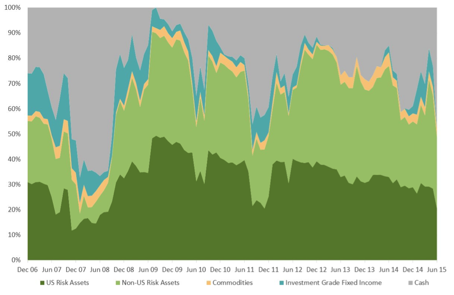
Over the history of our global balanced portfolio for US taxable investors, the Cash bucket has not yet been zero, but has ranged between 11% and 48%. On a simulated basis it reached a level of 67% in July 2008 and zero in August 2009 (although you cannot see this in Chart 1 below as data is shown every six months).

Chart 1 below shows how the desired asset allocation has changed over the life of our Fund (January 2012), and prior to that back to the start of 2007 (on a simulated basis prior to 2012). In separate back-tests from 1925 and 1975 to the present, the value and momentum dynamic asset allocation approach described in this note improved investment returns and decreased risk as compared to a comparable static Baseline portfolio. For more detail, please see the research note, “Investing for the Rest of Us.”

Chart 1: Historical Asset Allocation

At least once a year, we review our investment approach in detail, and consider improvements. We favor those that make our approach simpler and more intuitively appealing, which we hope will help us stay the course for the long term, and prevent ad hoc, subjective views making an unwanted entry into our process.

We hope this description of our methodology has left you with a clearer understanding of how we implement our Active Index Investing® approach. We have tried to go into enough detail so you can understand every aspect of our methodology, but please don’t hesitate to get in touch with any questions or suggestions you may have. We value your input.

---

Disclaimer:

The information contained on this page has been provided as general commentary and for information purposes only. It does not constitute any form of advice nor recommendation to buy or sell any securities or adopt any investment strategy mentioned therein. It is intended only to provide observations and views of the author(s) at the time of writing, both of which are subject to change at any time without prior notice. The information contained in the commentaries is derived from sources deemed by Elm Partners to be reliable but its accuracy and completeness cannot be guaranteed. This material does not have regard to specific investment objectives, financial situation and the particular needs of any specific person who may read it. It is directed only at professional investors as defined by the rules of the relevant regulatory authority. Any views regarding future prospects may or may not be realized. Past performance is no guarantee of future results.

---

1. Notice that the allocation to fixed income and cash in the Baseline portfolio is 25% as compared to 35% in the 65/35 simple target portfolio. The reasons for this are: 1) the Baseline is a more diversified and balanced portfolio and so should be able to support a smaller weight in fixed income and cash, and 2) as described below, our dynamic asset allocation approach can reduce risk more than it can increase it, due to our leverage constraint.