Introduction¹

This paper is meant to provide a comprehensive overview of Elm’s investment process for Separately Managed Account clients.² Our investment process is entirely rules-based and is intended to be understood by our investors, with no ‘black box.’ The philosophical foundations of our approach are laid out in our book The Missing Billionaires: A Guide to Better Financial Decisions, and we’ll reference passages from the book as we go along for those interested in additional information and detail.

The goal of The Missing Billionaires is to give modern investors a framework for making their own principled financial decisions pertaining to both investing and spending. The goal of Elm is to help you efficiently implement a portfolio to harvest the long-term returns available from broad public markets. We want your Elm portfolio to be consistent with the core ideas in the book, in sync with how you’d like to be investing, and appropriate for your individual financial situation.

One of the foundational concepts we discuss in The Missing Billionaires is called the Merton Share, for determining the optimal amount of wealth to invest in a risky asset or portfolio. [Ch. 2,3] The Merton Share is a ‘rule of thumb’ which, subject to a variety of assumptions,³ reflects that if you can invest in a risky asset with excess return \(\mu\) and volatility \(\sigma\), then the optimal wealth fraction to invest is proportional to \(\frac{\mu}{\sigma^2}\).

The Merton Share is a more flexible relative of the well-known Kelly Criterion. It’s derived from the theory of financial decision-making under uncertainty, and is more natural for sizing investments like stocks and bonds. [p. 37] As a rule of thumb, it isn’t appropriate to use directly in every situation, but nonetheless it provides an important core intuition: that we should want more of a risky asset when we’re getting more excess return relative to a safe asset (and vice versa), and also that we should want more of the risky asset when it has less risk (and vice versa).

Conceptually, Elm’s rules-based asset-allocation is simply trying to provide a practical, intuitive implementation of this principle across a universe of global asset classes which can be held through highly liquid, low-cost index ETFs. We provide three ‘Dials’, described below, which you can use to customize the implementation so it’s consistent with your personal risk aversion, preferences, and non-Elm investments.

Baseline Selection

Elm’s investment process begins with constructing your Baseline Portfolio from the asset classes below. This is the portfolio you’d want to hold in the Baseline Environment, where every major risk asset class has a 4% Risk Premium, and a ‘neutral’ risk level which is neither high nor low, but somewhere in between. Risk Premium is defined as the excess long-term return expected from the asset class above a safe asset return.

We divide the investment universe into the following categories and asset classes, and we use ETFs to invest in each asset class. We only use broad-market, low-cost index ETFs which are market-cap weighted. The weighted-average expense ratio across a typical portfolio is currently about 0.06% per annum. We’ve listed one of our preferred instruments after each asset class:

• US Risk Assets: US Broad Equities (VTI), US Value Equities (VTV), US Small-cap Equities (VB), US Real Estate (VNQ), US High-yield Bonds (HYLB)
• Non-US Risk Assets: Europe Equities (VGK)⁴, Emerging Markets Equities (VWO), Developed Asia Equities (VPL), Canada Equities (BBCA)
• Safe Assets: US TIPS (SCHP), US T-Bills (SGOV), US High-grade Nominal Bonds (BND), US Muni Bonds (MUB)

There are two Dials which you can use to choose the Baseline appropriate for you:

1. Risk Level Dial: The percentage of Risk Assets to hold in the Baseline Environment, with the rest held in Safe Assets. For example, a baseline level of 75% Risk Assets / 25% Safe Assets is a common choice. [Ch. 5, 12] The Baseline Safe Asset mix is 40% TIPS, 40% T-Bills, 10% Nominal bonds, and 10% Muni bonds (for taxable accounts).
2. Global Mix Dial: This determines how to divide the Baseline Risk Asset weight between US and non-US assets, in the Baseline Environment. The neutral setting, 0% on the dial, is an adjusted market-cap-weight mix⁵. A positive dial setting represents a bias toward US equities, for example +50% is halfway in-between the adjusted market-cap weights (which change over time) and 100% US equities. Similarly, -50% is halfway towards 100% non-US equities. Any setting between -100% and +100% is possible. A neutral setting of 0% in theory represents the most diversified, risk-efficient portfolio to hold, but you may also want to take into account the distribution of assets held outside your Elm portfolio, or express some degree of personal home bias.

There are no dial settings which are objectively optimal for all clients – the best settings for you will depend on your personal risk preferences and financial situation. You can tell us what settings you want, or we can help you figure out the settings most appropriate for you.

Dynamic Asset Allocation

The Baseline Portfolio specifies your ideal asset allocation in the Baseline Environment, a hypothetical state of the world with 4% Risk Premia and neutral risk level. We’re not assuming that 4% is the average Risk Premium equity markets will experience over time, it’s just a convenient reference point for establishing preferences in one state of the world.⁶ But of course actual Risk Premia and market risk levels are changing all the time, and Elm’s asset allocation is designed to adjust to changing market environments. For each risk asset class, we adjust the Baseline Weight to a Target Weight based on that asset class’s current level of Risk Premium and market risk. Portfolio weights must add up to 100%, and leverage and shorting are not allowed. Whatever isn’t being allocated to the Risk Asset classes is split up amongst the Safe Assets.

Using the Dynamic Scaling Dial, you can specify how dynamically Elm responds to changes in the market environment. With 100% Dynamic Scaling, Risk Premium deviations cause the Target weight to vary from the Baseline by the same proportion as the Risk Premium varies,⁷ with a maximum variation of ±2/3 the Baseline Weight. Changes in market risk level will cause the Target Weight to vary by either +1/3 or -1/3 the Baseline Weight.⁸ Setting the Dynamic Scaling Dial to a lower level will cause all the variations to reduce correspondingly, until at 0% Dynamic Scaling the Target Weights will always equal the Baseline Weights.

In implementing Elm’s dynamic scaling, our Risk Premium metric for a broad equity market is 1/CAPE – 10y TIPS Real Yield. CAPE is the Cyclically-Adjusted PE Ratio popularized by Robert Shiller. 1/CAPE is a forecast for the long-term real return of equities, and the 10y TIPS Real Yield is our preferred proxy for the long-term safe asset return. [p. 50]

For the market risk level, instead of measuring this directly, practical considerations have led us to use as a proxy a one-year momentum signal, which measures whether the market is above its one-year moving average (low risk), or below it (high risk).⁹ Using momentum as a proxy for market risk level is consistent with momentum-scaling and volatility-scaling producing very similar results when applied to equity markets.¹⁰ We use a momentum signal to vary the mix of Safe Assets as well, for example with 100% Dynamic Scaling if TIPS price momentum is positive we’d hold 60% of Safe Assets in TIPS (vs. the 40% Baseline mix), or 20% if TIPS price momentum is negative.

Below we show an example of Elm’s dynamic asset allocation for US Equities and 100% Dynamic Scaling as of 10/31/2005:

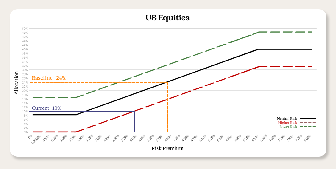
In this example, the baseline weight for US equities is 24% and the Target Weight is 10%, because:

• The current risk premium is about 3%, or 3/4 the Baseline level of 4%. Adjusting the Baseline weight by the same proportion yields 18% = 24% * 3/4.
• The current market is in a higher-risk state, because momentum is negative, so we adjust the target weight by -1/3 the Baseline Weight. This results in a final Target Weight of 10% = 18% – (1/3) * 24%.

At the extremes, 100% Dynamic Scaling can result in dramatic departures from the Baseline Portfolio, with as much as 100% or 0% in equities. For example, from 1990-2023, the total equity allocation would have varied from a low of 10% to a high of 100%, given a 75% Baseline Risk Level and neutral global mix. With 100% Dynamic Scaling, we expect a tracking error of portfolio returns vs. the Baseline Portfolio of about 6% per annum over long periods of time.¹¹

With 50% Dynamic Scaling, the dynamic deviation from the Baseline Portfolio will typically be half as large as that above, given the same state of the world.¹² The tracking error vs. Baseline will also be roughly half as large. If you have sensitivity to extreme allocations, or to under-performance relative to the Baseline Portfolio, a Dynamic Scaling of 50% may be a good choice – it preserves many of the attractive benefits of a dynamic asset allocation, while resulting in less extreme portfolios with less tracking error. You can set the Dynamic Scaling Dial anywhere between 0-100%, but we suspect 50% or 100% will be the right choice for most individual clients. For clients who want a managed portfolio with a static asset allocation, we’re happy to accommodate that as well with a 0% Dynamic Scaling setting.

While not a literal implementation of the Merton Share in a multi-asset world, Elm’s dynamic scaling is clearly recognizable as being generally consistent with the Merton Share’s call for asset allocations to scale proportionally with risk premia, and inversely with market risk level. We think Elm’s implementation of dynamic scaling strikes the right balance between simplicity, robustness, and theoretical consistency.

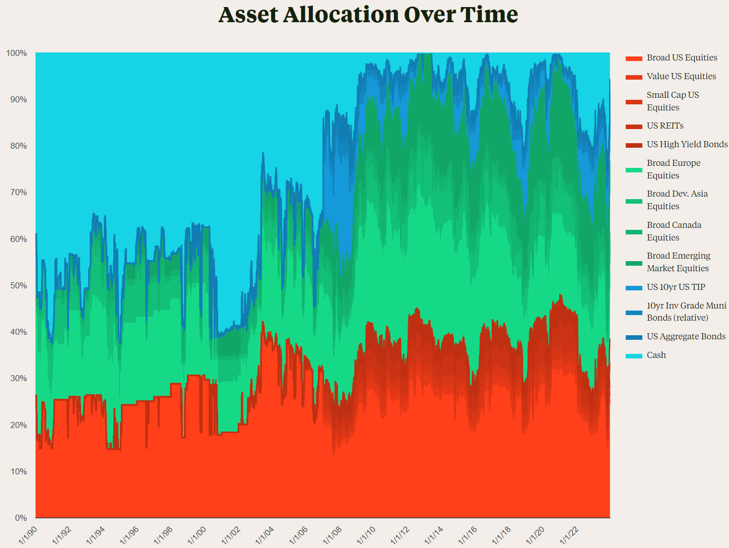
Here is the 1998-2023 history of the Target allocation, for a 75% equity baseline, neutral global mix, and 50% Dynamic Scaling:¹³

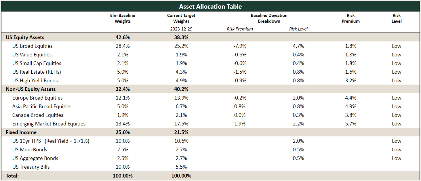
And here we show as an example Elm’s asset allocation as of 12/29/2023, for a 75% equity baseline, neutral global mix, and 50% Dynamic Scaling:

We don’t update the tables in this document, instead we provide a ‘live’ online tool which can be used to track the history of Elm asset allocations and their underlying details, for any combination of Dial settings: Asset Allocation Viewer.

Execution

Fees
Elm’s Investment Management Fee is 0.12% per annum, charged monthly in arrears on the average account balance over the month.

Custody
Your assets can be custodied at Fidelity or Schwab in a Separately Managed Account (SMA), or in certain circumstances JP Morgan. Your assets will always stay in your own name, and we set up client accounts so that only you have money and asset movement authority. We only have trading authority on the account, and we can be removed from the account at any time.

We can manage a wide variety of account types, including Individual, Joint, Trust, IRA, UTMA, LLC, LTD, Non-prototype Retirement, and certain self-directed 401(k) accounts. We can also manage accounts tax-efficiently for clients who are both US and UK taxpayers.

You can add new funds to Elm-managed accounts and we’ll typically get them invested next business day¹⁴, and you can remove funds anytime with two business-days notice. There are no lock-ups and you can remove Elm as a third-party manager on your account at any time.

Rebalancing
We divide each account into four sub-portfolios, and rebalance one sub-portfolio each week. This means that new market conditions take four weeks to fully filter though to the portfolio, but begin filtering through within a week. This significantly reduces the idiosyncratic risk associated with when we choose to rebalance.

Every week when we rebalance the sub-portfolio, we don’t just go right to the Target Weight for each asset class – that would generate an unnecessary trade volume, and would be tax-inefficient for taxable accounts. Instead, we run an execution optimizer which tries to find a parsimonious set of trades which mutually:

• Minimizes deviations from Target Weights
• Minimizes realized gains
• Maximizes realized losses
• Minimizes transaction costs
• Strictly avoids wash-sales from taxable to non-taxable accounts, and minimizes wash sales between taxable accounts¹⁵

On any given week, we could do several trades or no trades. At Fidelity and Schwab, ETF trading commissions are $0¹⁶, and we execute either market-on-close or VWAP over most of the trading day, so we believe that market-impact costs are de minimis.

Tax Efficiency and Tax Loss Harvesting
Elm’s dynamic asset allocation has the potential for high turnover, but this isn’t necessarily tax-inefficient as the turnover can generate realized losses roughly as often as realized gains, and we also perform regular tax loss Harvesting. In this note, we take a five-year period in which there were high market returns, and see that Elm’s dynamic asset allocation resulted in a slightly lower effective tax rate compared to a static asset allocation.

Elm automatically checks for and executes suitable tax loss Harvesting opportunities weekly. Harvesting using ETFs is highly efficient, as for most asset classes there are multiple high-quality, low-cost ETFs which are an acceptable replacement for one another. There is real tracking error between the replacement ETFs, otherwise replacing would trigger a wash sale, but the added risk from harvesting with ETFs is significantly less than from tax loss harvesting with individual stocks.

For those desiring additional expected harvesting, there is an account option to split the US Broad Equities asset class into subsidiary sectors and hold an ETF for each sector. This roughly doubles the number of instruments and trades in the account, and will result in a modestly higher amount of expected harvesting, because the dispersion across sectors is higher than that of the total market index.

Evaluating Elm

We expect that using Elm’s dynamic asset allocation will in the long run result in modestly higher expected risk-adjusted returns, compared to the Baseline Portfolio. However, due to the intrinsic noisiness of financial markets, it can be very challenging to accurately measure investment quality differences over the typical 1-10 year holding periods for which most people look at their account performance. We explore this in detail in our note What’s Past is NOT Prologue, in which we see that it takes vastly more than 10 years of data to reliably distinguish between two strategies of modestly different quality. Theory, reason, and history have combined to give us a strong prior belief about the merits of Elm’s approach, and Bayesian analysis can be used to update our beliefs in light of new information. Here are a few additional suggestions for how you can evaluate your Elm portfolio:

• Is your Elm portfolio making it easier for you to achieve and stick with diversified, broad public markets exposure?
• Is your portfolio aligned with your personal preferences and financial situation? Are there different dial settings which would make it better aligned?
• Is your portfolio improving the diversification and efficiency of your overall investing?
• Are your portfolio’s asset allocation, activity, and costs consistent with what you’d expect based on this paper and your discussions with us?

We note that one of Elm’s goals is not to generate higher returns compared to the S&P500, or whichever market index is doing the best over a given period. Setting aside whether this can be consistently achieved net of fees and risk costs, attempting to do this generally involves some combination of taking more risk and accepting less diversification, and all of Elm’s choices are going in the other direction. The benefits of lower risk levels and greater diversification are harvested primarily through being able to maintain larger fractions of your wealth invested in risky assets [p. 59], through avoiding high fees and other costs, and through your spending policy [p. 132-141].

Account Options

In addition to the Dials described above, clients can specify the following options for SMA accounts:

• Non-taxable: The account will be rebalanced without regard to realized gains/losses, will not conduct tax loss harvesting, and will not hold Muni bonds.
• US Sectors: Instead of holding Broad US Equities through a single ETF like VTI, your portfolio will hold each of the component sector funds which add up to the Broad US index. This somewhat increases account complexity and transaction volume, while also creating the potential for greater tax loss harvesting, because the sectors typically have greater dispersion than the total-market index.
• US/UK: For dual US/UK taxpayers. The account will only hold HMRC-reporting ETFs.

For clients who are not US taxpayers, we also have a Cayman fund, Elm Partners Portfolio Ltd, which has a Baseline of 65% Global Equities, 5% Commodities, and 30% Global Fixed Income. The Fund generally uses the same type of asset allocation rules described in this paper, and the prospectus is available upon request.

Getting Started

The easiest way to get started with Elm is through our Online Onboarding. For information related to account onboarding, you can also contact Mike Fothergill at mike@elmwealth.com. For more information or other questions about investing with Elm, please contact Elm’s CEO James White at james@elmwealth.com.

---

1. The content on this page is being provided for educational purposes only. It does not constitute any form of investment advice, or any form of recommendation to buy or sell any securities or adopt any investment strategy mentioned herein. This material does not have regard to specific investment objectives, financial situation and the particular needs of any specific reader. Any views regarding future prospects may or may not be realized. Past performance is no guarantee of future results.
   
2. The investment process for clients in Elm’s legacy US private fund EPP LLC, and Cayman private fund EPP Ltd for non-US investors is grounded in the same philosophy, but many specific implementation details differ.
   
3. Specifically that you’re trying to maximize CRRA utility, you can only invest in the risky asset or risk-free asset, returns are normally distributed, and you can continuously rebalance.
   
4. Including UK
   
5. We start with the global market cap weights, then modestly adjust for US home-bias, and regional GDP and Earnings weights. The latter adjustments can help mitigate extreme valuations such as those seen in ’80s Japan equities, causing one market to implausibly dominate the baseline.
   
6. Under the hood it’s not exactly 4% for each asset class, to ‘even out’ differences between the markets, so the 4% thought experiment is still valid.
   
7. This is the variation most consistent with the Merton Share.
   
8. With a narrow transition zone in-between for when risk level is close to neutral
   
9. Adjusted for inflation, dividends, and risk premium.
   
10. See our note Steadfast, Greedy, or Fearful for more on this topic.
    
11. By tracking error, we specifically mean the standard deviation of the difference between annual portfolio and baseline returns. For any particular year or period, differences significantly larger than the expected tracking error are quite possible, as we do believe the distribution of tracking error is not well-represented by the normal distribution.
    
12. The exception being in periods where the no-leverage constraint is binding.
    
13. 1998 is the first full year for which TIPS real yields are available. We begin the TIPS/T-Bills/Nominals/Munis Safe Asset mix in 2007.
    
14. If greater than $50k, or on our weekly rebalancing cycle otherwise.
    
15. We allow small wash sales between taxable accounts if they help with another element of the trade optimization, as the loss is not permanently lost.
    
16. Up to 10,000 shares at Fidelity.