By Victor Haghani and James White ¹

March 2020 packed 2 ½ years of normal U.S. stock market volatility into one month, making it the most volatile month on record. Daily variability clocked in at 6%, six times higher than the average over the past 90 years. How should an investor respond to such volatility? There are at least three schools of thought:

1. Steadfast: Stay the course and don’t be shaken by short-term swings in volatility. When setting your asset allocation to begin with, assume that the stock market will be much more volatile than normal from time to time, and when that happens take it in stride. As Vanguard founder John Bogle said, “Don’t pay a lot of attention to the volatility in the marketplace. All these noises and jumping up and down along the way are really just emotions that confuse you.” ²
2. Greedy: Increase your exposure to the market, because, as Warren Buffett has counseled, “Be fearful when others are greedy and greedy when others are fearful.”
3. Fearful: Reduce your exposure to the market because it has become riskier right now. This approach, known as “Volatility Targeting,” has been researched and supported by a host of respected academicians, with Ray Dalio, founder of the Bridgewater hedge fund group, its highest profile practitioner.³

Let’s work through these arguments in a world of two investments: a risk-free asset and the stock market. Let’s say you’re an investor who has just retired and has wealth well in excess of what’s needed to provide the basics for your family.⁴ How much you would optimally allocate to the stock market depends on your estimate of its return and risk relative to the risk-free asset, your personal degree of risk aversion, and how much savings you need to set aside to meet basic needs.⁵ As we’ll discuss below, which of the three schools of thought will appeal to you most will depend primarily on where you look for your estimates of expected risk and return.

Steadfast

Many investors and researchers use long-term market history to extrapolate future expected returns. This is the foundation of the Bogle recommendation: assume long-term return and risk are constant and ignore changes in short-term volatility and valuation metrics. We’re generally skeptical of backward-looking, historically-based forecasts of the future, though Bogle’s counsel is easy to follow and has the potential psychological advantage of helping an investor look through times of stress and turmoil. Most proponents of the steadfast approach recommend periodic portfolio rebalancing to maintain static target asset allocation weights.⁶

Greedy

A more adaptive, and forward-looking approach acknowledges that the long-term expected return of the market varies over time. Among the most commonly used, and effective, estimators of the future return of the stock market is the Cyclically-Adjusted Earnings Yield popularized by Robert Shiller. Importantly, it’s a predictor of the very long-term market real return, ignoring the hard-to-predict changes in sentiment that dominate shorter-term returns. If we rely on this long-term estimator, then it follows we should want to use a similarly long-term measure of risk, which will be relatively unaffected by swings in short-term volatility.⁷ This is consistent with Buffett’s advice to be greedy when others are fearful: when the stock market goes haywire and drops precipitously, long-term expected returns have likely gone up, while long-term risk is little changed.

Fearful

“The long run is a misleading guide to current affairs. In the long run, we are all dead. Economists set themselves too easy, too useless a task if in the tempestuous seasons they can only tell us that when the storm is long past the ocean will be flat.”
  – J.M. Keynes, A Tract on Monetary Reform (1923)

While the “Earnings Yield” estimate of the market’s long-term return is based on expected cash flows in the form of earnings and dividends, in the short run, stocks are driven primarily by changes in how market participants discount those future cash flows. As Benjamin Graham put it: “In the short run, the market is a voting machine but in the long run it is a weighing machine.” A Volatility Targeting strategy scales exposure inversely to short-term market volatility, increasing exposure when volatility is low and decreasing it when volatility is high. There are several lines of thought which support Volatility Targeting.⁸ Many practitioners focus on the desirability of keeping portfolio volatility constant over time, which may give investors greater peace of mind and potentially the confidence to take higher levels of risk over time. Indeed, Volatility Targeting is the optimal strategy under the assumption that the Sharpe Ratio (i.e. return-to-risk ratio) of equities stays constant as short-term volatility varies.⁹ Another popular theory suggests the market systematically under-reacts to changes in short-term volatility.¹⁰ The idea is that when an asset’s short-term volatility goes up, investors are slow to mark down its price enough to make the expected short-term return high enough to warrant holding as much of that asset. By reducing exposure when volatility goes up, the volatility-targeter seeks to get ahead of the slow but necessary mark-down process.

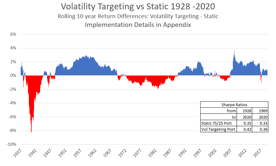
In practice, there are many impactful details to implementing a Volatility Targeting strategy, which is why historical studies reach varying conclusions on its effectiveness. We found that studies which assume the least practical implementations for ordinary investors produced the most attractive historical results. The chart below is based on how we imagine an individual investor with a baseline asset allocation of 75% US equities and 25% T-bills might actually apply Volatility Targeting, with no leverage and rebalancing each month-end. Please see the Appendix for full details of all historical backtests. The Volatility Targeting strategy did well from 1985 to the present, but less so over the entire period. We explored a wide range of different implementations and none that we could find was significantly better than what’s displayed below.

A Different Shade of Fearful: Momentum

“…most of the time the trend prevails…. Most of the time we are punished if we go against the trend.”
  – George Soros, Soros on Soros: Staying Ahead of the Curve

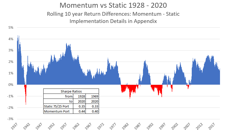
There is another indicator of short-term returns that has a loyal group of followers, and has some strong similarities with Volatility Targeting: Momentum. Time Series Momentum is measured by comparing today’s market level to a reference point, usually 6 – 12 months in the past for asset allocation purposes. If Momentum is positive, meaning today’s level is higher than its recent average, it indicates that near-term returns will be higher than if Momentum is negative. Researchers have found that Momentum is predictive of near-term asset price performance across virtually all assets that have been investigated.¹¹ There are many theories for why Momentum has worked; nearly all are based on behavioral foibles, grounded in the tendency of investors to extrapolate recent performance. The result is “return-chasing” behavior, creating trends in asset prices that Momentum indicators identify as they start to unfold. The chart below shows that a Momentum-driven portfolio performed quite a bit better than a static portfolio historically. In all 9 decades from 1930 to 2020, the 10-year return on the Momentum portfolio was higher than the static portfolio, with roughly the same risk (please see Appendix for more detail).

Volatility Targeting versus Momentum

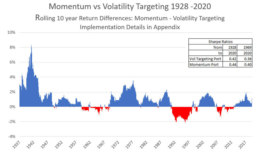
Researchers have long noticed that volatility tends to rise when the stock market falls, and vice versa, which suggests that for equities Volatility Targeting and Momentum signals tend to line up most of the time.¹² We found that from 1928 – 2020 they in fact did point in the same direction 67% of the time. The chart below shows that over this period Momentum pretty consistently out-performed the Volatility Targeted dynamic portfolio. In 8 of the 9 decades from 1930 to 2020, the 10-year return on the Momentum portfolio was higher than the return on the Volatility Targeted dynamic portfolio, with the same risk over the past 50 years, and slightly higher risk over the full period. The Momentum portfolio also had a modestly higher Sharpe ratio.

We emphasize that such backtests do not by themselves provide enough evidence to warrant applying either approach, or preferring one to the other: past returns do not indicate future performance. We always need to ask whether the historical patterns we have found are the result of randomness, structural features, or systematic investor behavior. Even if we believe it’s not the result of chance, we need to also believe it’s likely these behaviors will persist in the future and outweigh the actions of other investors who are trying to take advantage of them.

Looking past the historical data, if you believe investors are focused on short-term return and risk, and are slow to adjust prices to changes in volatility, then you may be more attracted to Volatility Targeting, even though Momentum has historically done better as an indicator of short-run returns. However, if you are more attracted to the paradigm that return-chasers drive market dynamics, then you’ll find Momentum an attractive indicator to use in scaling your exposure to the market. Of course they are not mutually exclusive, and you may want a blend of both strategies. One good question to ask is whether you believe that high volatility in a rising stock market would have the same predictive power as high volatility in a falling market. Is it high volatility or the market’s recent direction that is primarily driving near-term returns? ¹³

Finally, even if you view Volatility Targeting and Momentum as equally likely to improve the risk-adjusted return of your portfolio, you may also want to consider the relative complexity of implementation, which favors Momentum as the strategy with fewer choices to make.

Conclusion

What does all this mean for how you should respond to extreme market volatility? Depending on how you think about long-term and short-term returns, and your desire for simplicity in managing your savings, we see merits in all the schools of thought, individually or in any combination. At Elm, we favor a fusion of Buffett’s approach for determining our long-term allocation to equities with Soros’ advocacy of Momentum to adjust for investors’ penchant to chase returns in the short term.

---

Appendix: Details of Historical Performance of Volatility Targeting, Momentum and Static Portfolios

Data
We used daily S&P 500 index price data from finance.yahoo.com using the series ^GSPC. We used dividend and US CPI data from Professor Robert Shiller’s website to create a real total return index for the US stock market from December 31, 1928 to March 27, 2020. For T-bills, we also used Robert Shiller’s online data, using the one-year T-bill rate as a proxy for a daily T-bill rate. For the real return of the static portfolio, we assumed the portfolio was held at a constant asset allocation of 75% equities and 25% T-bills, rebalanced back to those weights at the end of each month. We assumed no transactions costs or frictions of any kind in these historical analyses. The data table below has an estimate of turnover for each of the portfolios.

Volatility Targeting
For the Volatility Targeting portfolio, we used the historical average 60-day rolling US equity volatility over the whole 1928 – 2020 period of 16.5% as the target level of volatility at which the portfolio will be 75% allocated to equities.¹⁴ For our base case, we set the allocation to equities, W* = 75% * 16.5% / Vol , where Vol is equal to annualized volatility of equity returns over the past 60 trading days. One way of thinking about this form of Volatility Targeting is that it assumes that in the short term the Sharpe Ratio of the equity market stays constant by the expected return of equities changing in proportion to changes in short-term volatility. As an illustration of the application of this rule, at the time of writing 60 day realized volatility was 63% pa, calling for an allocation to equities of 20%. We imposed a no-leverage constraint by capping the desired allocation to equities at 100%. The average allocation to equities over the whole period was 82.2%, higher than the 75% static baseline. The quality of historical returns measured by Sharpe Ratio is not materially changed by different choices target level of volatility. We also ran historical simulations using 20-day and 40-day lookback windows, squeezed volatility estimates in the spirit of GARCH analysis, and also we used VIX implied market volatility from 1990 onwards, the period over which VIX data was available. None of these choices for estimating market volatility as an input to the asset allocation rule made the historical returns of Volatility Targeting materially different. It is not surprising that using implied volatility didn’t materially improve the results of Volatility Targeting. Since 1990, one-month implied volatility has explained about 50% of next month’s realized volatility, about the same predictive power we get from predicting next month’s realized volatility using the past month’s realized volatility. We also explored using the Merton Rule at the end of each month to set the target allocation to equities, W* = μ / γ / σ² , which is consistent with the assumption that the short-term expected return of equities remains constant despite changes in short-term market volatility. This is referred to as “Variance Targeting.” We held the expected excess return, μ , constant at 5%, the coefficient of risk aversion, γ constant at 2.5,¹⁵ and volatility, σ , equal to the past 60 business days’ realized stock market volatility. We chose these parameters for their reasonableness and as they result in an average asset allocation not too far from the static baseline target of 75% equities. This approach also did not materially improve the quality of returns versus our baseline Volatility Targeting parameterization. We explored daily rebalancing, which roughly quadrupled turnover, without a material increase in quality of returns. We relaxed the leverage constraint to allow the investor to hold up to a 4x leveraged exposure to equities (an implementation we strongly advise against), but again this did not materially change the Sharpe Ratio of the strategy, although it did materially increase absolute historical returns. The only assumption which substantially improved the performance of Volatility Targeting was the unrealistic presumption that the investor had perfect foresight with regard to future realized volatility.¹⁶

Momentum
Momentum was measured as the current total real return index less the average of the total return index over the past year less 2.5%. The purpose of subtracting 2.5% is to make the incidence of positive and negative Momentum roughly equal. The target allocation for the Momentum portfolio was set at the end of each month as 100% equities/0% T-bills if Momentum was positive, and 50% equities/50% T-bills if Momentum was negative. We also used a Momentum signal based on a six month look-back window, and the results were similar to those from the one-year lookback. The average allocation to equities over the whole period was 79.2%, higher than the 75% static baseline, and lower than the average 82.2% equity exposure in the Volatility Targeting strategy.

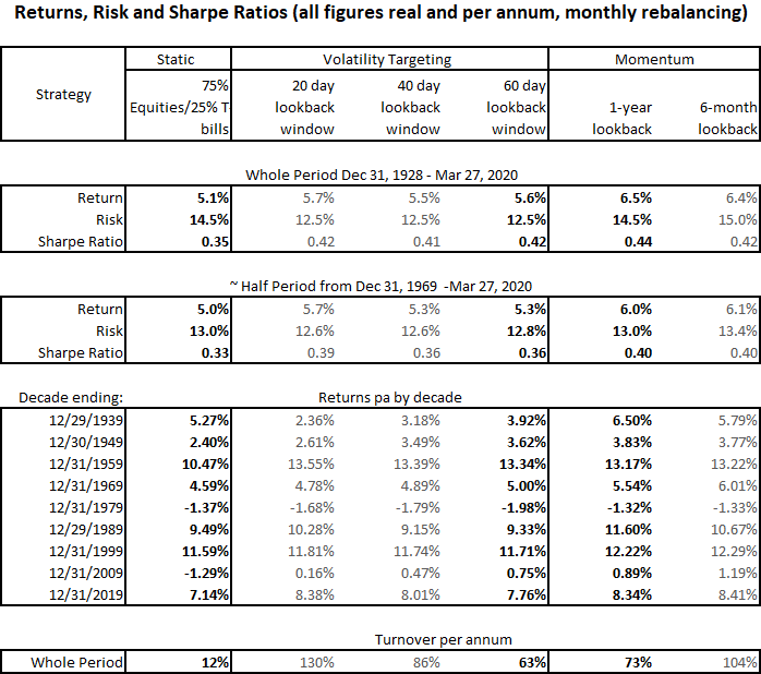
The table below provides further details of the historical simulations explored.

---

Further Reading and References:

• Black, Fischer. “Studies of Stock Price Volatility Changes.”  Proceedings of the 1976 Meeting of the Business and Economic Statistics Section, American Statistical Association, 177-181. 1976.
• Engle, R. “Autoregressive Conditional Heteroskedasticity with Estimates of the Variance of U.K. Inflation.”  Econometrica 50: 987–1008, (1982).
• Fleming, J., C. Kirby and B. Ostdiek. “The Economic Value of Volatility Timing.”  The Journal of Finance 56 (1): 329–352. 2001.
• Fleming, Jeff, Chris Kirby and Barbara Ostdiek, “The economic value of volatility timing using realized volatility.”  Journal of Financial Economics 67, 473–509. 2003.
• French, Kenneth R., G. William Schwert and Robert F. Stambaugh. “Expected Stock Returns and Volatility.”  Journal of Financial Economics 19, 3–29. 1987.
• Geczy, Christopher and Mikhail Samonov. “Two Centuries of Price Return Momentum.”  Financial Analysts Journal, Vol. 72, No. 5. Sep 2016.
• Harvey, Campbell R., Edward Hoyle, Russell Korgaonkar, Sandy Rattray, Matthew Sargaison and Otto Van Hemert. “The Impact of Volatility Targeting.”  Journal of Portfolio Management. Fall 2018.
• Lochstoer, Lars and Tyler Muir. “Volatility Expectations and Returns.”  INSEAD. 2019.
• Merton, Robert. “Lifetime Portfolio Selection under Uncertainty: The Continuous-Time Case.”  The Review of Economics and Statistics, Vol. 51, No. 3. Aug. 1969.
• Moskowitz, Tobias, Yao Hua Ooi and Lasse Heje Pedersen. “Time Series Momentum.”  Journal of Financial Economics. 2012.
• Tang, Yi, and Robert F. Whitelaw. “Time-varying Sharpe ratios and market timing.”  Quarterly Journal of Finance 1, 465–493. 2011.

---

1. This not is not an offer or solicitation to invest, nor should this be construed in any way as tax advice. Past returns are not indicative of future performance.
   We thank Antti Ilmanen, Campbell Harvey and Myron Scholes for their helpful comments. Of course, the views, analysis and any errors are solely our own.
   
2. MarketWatch: Why Bogle and Buffett tell investors to ignore market noise
   
3. In a 2010 white paper titled “Engineering Targeted Returns and Risks,” Dalio explained “how to structure a portfolio to target a 10% return with 10-12% risk.” While Bridgewater’s Volatility Targeting implementation is proprietary, it is believed that they use longer-term measures of volatility, which would dampen their reaction to changes in volatility over the short run.
   
4. Or, if you’re still working, you have a secure job that makes your human capital very low risk and stable, like a government bond.
   
5. Robert Merton provided an early solution to this problem:
   W* = (μ – r) / (γσ²)
   where W* is the fraction of wealth in excess of subsistence needs to allocate to the risky asset, μ is the expected return of the risky asset, r is the risk-free rate, σ is the expected variability of the risky asset and γ is the investor’s level of risk aversion. See our note Measuring the Fabric of Felicity for a deeper discussion, particularly of γ .
   
6. Some would argue that maintaining static weights is an active strategy, in that it calls for buying equities when they fall and selling when they rise. One’s choice of benchmark against which to measure other investment approaches is important and can have a significant influence on the selection of the optimal strategy. For example, see our recent note: Back to the Future: Reviving a 19th Century Perspective on Financial Well-Being, in which we argue that an investor’s choice of minimum risk asset will have a profound influence on portfolio choice.
   
7. Let’s take an investor with a 25-year planning horizon. He believes stock market volatility will be 18% a year in the long run, and it’s been running at 18% in the short run. But then all of a sudden, there’s a panic and one-month volatility (i.e. VIX) goes to 50%. But he expects volatility to drop half-way back to 18% in a couple of months. Under these assumptions, the short-term spike in volatility would only raise 25-year expected volatility from 18% to 18.5%.
   
8. See French et al. (1987), Fleming et al. (2003), Tang and Whitelaw (2011), Harvey et al. (2018), Lochstoer and Muir (2019).
   
9. Optimal under the Merton Rule. For a slightly different perspective, invoking the concept of time-diversification, see this interview with Myron Scholes.
   
10. Lochstoer and Muir (2019) state: “Slow moving expectations about volatility lead agents to initially underreact to volatility news followed by a delayed overreaction.”
    
11. See Moskowitz et al. (2012) and Geczy and Samonov (2016).
    
12. First noted in Black (1976). Harvey et al., pp14, 31 (2018):
    “Risk assets exhibit a so-called leverage effect (i.e., a negative relation between returns and volatility), and so volatility scaling effectively introduces some Momentum into strategies. That is, volatility often increases in periods of negative returns, causing positions to be reduced, which is in the same direction as what one would expect from a time-series Momentum strategy. Historically such a Momentum strategy has performed well…we show that it is indeed the Momentumness of volatility scaling that explains a large part of the cross-sectional variation in the Sharpe ratio improvement when using volatility scaling for the various assets considered.”
13. An example of one such period to consider is the five year period starting in late February 1932, during which the S&P 500 experienced a real total return of 23.5% per annum, with realized volatility of 35%.
    
14. Realized volatility over the whole 1928 – 2020 period, measured using daily data was 19.3%, higher than the overlapping 60 day realized volatility was 16.5%. This difference is mostly due to the distribution of daily returns being significantly fat-tailed versus a standard normal distribution.
    
15. See our note Measuring the Fabric of Felicity for a discussion of the coefficient of risk aversion.
    
16. Perfect foresight is highly beneficial in nearly all realms of investing, and we commend its use whenever possible.