To Realize, or Not to Realize Elm Partners

October 22, 2020

Taxes

To Realize, or Not to Realize

By Victor Haghani and James White ¹

This is a note about taxes, however: we are not tax experts and
nothing in this note should be construed as tax advice.

With the US presidential election just a few weeks away, it’s a good time to think about capital gains taxes. A number of our clients have been concerned about the possibility of significantly higher tax rates in the future and have asked us how we think about the investing implications of such a change. In this note, we suggest a framework based on maximizing expected risk-adjusted wealth for answering some of the important questions arising from the interaction of taxes and investing.² We believe this framework is superior to a conventional static analysis, and we’ll explain why as we dive into the central question arising from tax rates potentially increasing in the near future: to realize gains now, or to defer realization to the future.

Investment theory holds that in a world of efficient markets, random walks and no taxes, horizon shouldn’t materially affect many types of investment decisions. However what we have found is that as soon as tax enters the picture, horizon in many situations becomes the single most important input an investor needs to think about. We find that for investors with long horizons and moderate-size unrealized capital gains, it will usually make sense to defer realization even if the investor expects the tax rate to jump by 20 percentage points. We were surprised to find that at intermediate time horizons, the optimal decision can be to realize some, but not all, of the unrealized gains. Investment horizon isn’t the only critical input, and the interaction of all the relevant variables puts the development of a generic rule-of-thumb out of reach. Optimal decision-making in light of taxes is a function of many idiosyncratic and personal inputs, which is why we decided to provide a calculator you can use along with the note.

You can find our Decision Calculator here.
You can find the math and code behind the framework here.

The central question we will address in this note is whether it is better to sell (and re-purchase) appreciated assets now and pay today’s long-term capital gains tax rate, or wait to realize gains in the future and pay a likely higher capital gains tax rate.

At first, this may seem like a fairly straightforward problem of weighing a bigger payment in the future against a smaller payment today: simply a question of the time value of money using an appropriate discount rate.³ In many circumstances, the decision would ride on a choice between different plausible discount rates. For example, in the base case we’ll discuss below, we’d want to realize early if we chose the risk-free interest rate, while we’d defer realization to the horizon if we used the expected return of a plausible risky asset. But as we’ll explain in this note, there is no robust way to choose an appropriate discount rate in a static framework. There are three main problems with the conventional approach, which all arise from the fact that risk is an integral part of the problem:

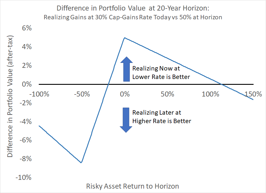
The conventional analysis captures only one of many possible scenarios. For example, the asset may drop below its cost basis resulting in no tax liability in the future, as the government doesn’t pay us “negative taxes” when we have a capital loss.⁴ A sound analysis needs to take account of all possible outcomes. Chart 1 shows how realizing gains now vs. later can result in dramatically different changes in value depending on the final level of the risky asset at the investment horizon.⁵
Considering many possible scenarios and making decisions which maximize your expected wealth still may not lead us to the correct decision. The problem is that maximizing expected wealth leads to absurd decisions around risk-taking: for any investment with a positive expected return above the risk-free rate, investing more in that investment will always lead to higher expected wealth, so it can’t help to answer any questions involving trade-offs between risk and return.⁶
The conventional static comparison, by construction, cannot find that a partial realization of gain is optimal, even though (as we’ll see below) there are cases when that’s exactly what an investor should do.

In addition, although of lesser impact, the static analysis doesn’t take into account the effect a higher future tax rate may have on how much of the risky appreciated asset you want to hold going forward, nor can it determine how tax rate uncertainty impacts the optimal allocation decision.

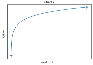
The goal in sound financial decision-making is to make choices which offer the best risk-adjusted result. This requires accounting both for uncertainty in outcomes and for the decision-maker’s personal level of risk-aversion. The standard approach to quantifying an individual’s aversion to risk is through their utility function: a mapping between wealth and the benefits of wealth, its utility. Classical utility functions show utility increasing with wealth – but as wealth increases, it produces diminishing marginal gains in utility, as illustrated in Chart 2. This has a deep connection to risk-aversion and risk-taking: given a risky situation, the more your loss of utility is disproportionately large relative to a potential gain, the more compensation you require to bear that risk. Thus, the more concave the utility curve, the more risk-averse the individual.

To make good risk-adjusted decisions, we need to find choices which maximize an individual’s expected utility, not expected wealth.⁷ There’s a direct correspondence between utility and risk-adjusted wealth (they’re interchangeable) – so going forward, we’ll perform our calculations using utility, and then express our results in terms of risk-adjusted wealth. That will allow us to compare different decisions in dollars rather than units of utility, which some readers may find too abstract. Armed with this tool, and assuming a typical degree of investor risk-aversion, we can determine to what extent we should realize a capital gain at the lower tax rate today.⁸

To do this, we calculate expected risk-adjusted wealth for each possible amount of immediate realization and each possible allocation to the risky asset, as follows:

For each possible price of the risky asset at the investment horizon, we calculate how much after-tax wealth the investor would have.⁹
We use the investor’s utility function to translate that amount of after-tax wealth into personal utility.
We multiply each amount of utility by the probability of the risky asset realizing the corresponding price at the horizon, using the risky asset’s assumed expected return and risk. We add up the probability-weighted utility values, and this gives us expected utility.
Using the investor’s utility function, we translate from expected utility into risk-adjusted wealth.

The result is an Expected Risk-Adjusted Wealth curve as a function of how much gain to realize immediately, given an optimal allocation to the risky asset.

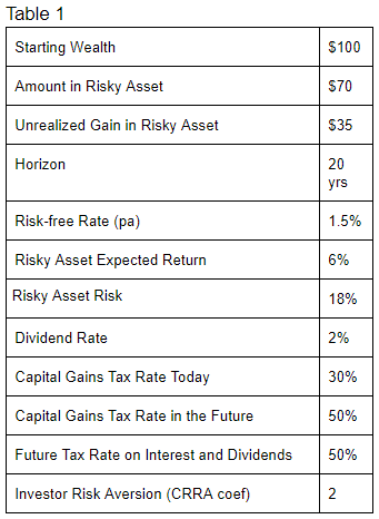
To illustrate this analysis, we’ll assume the investor has a 20-year horizon, that the risky asset (a stock ETF, for example) has an expected return of 6% with 18% volatility, and that the long-term capital gains tax rate will go from 30% today to 50% in the future. We’ll also assume that the investor must pay tax at the horizon, without the benefit of tax mitigations such as step-up basis for estate and charitable purposes, 1031 exchanges or moving state tax jurisdictions (although all of these could be modeled within this framework).¹⁰ If the investor has a capital loss at the horizon, we assume a zero value for the loss carryforward. The full set of assumptions are in Table 1.

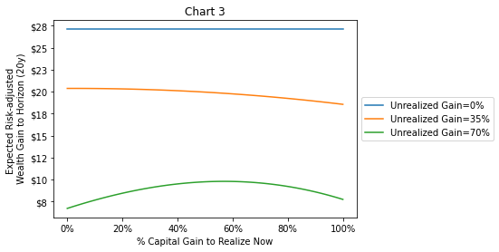
Chart 3 displays the risk-adjusted wealth curves for different initial levels of current unrealized gain, assuming an optimal risk allocation and a starting portfolio worth $100 (ignoring the tax liability). These curves allow us to find the decision – the percentage of gain to realize today – that maximizes expected risk-adjusted wealth. For an asset with 0 initial unrealized gain (blue), whether we sell the asset now or later doesn’t matter as there is no gain to realize; as expected, we see expected risk-adjusted wealth is constant. For our base-case unrealized gain of 35% (orange), realizing nothing now produces the highest gain in expected risk-adjusted wealth of approximately $20.5, the leftmost point on the curve. If the investor instead chose to realize all gains today, the rightmost point on the orange curve, their expected risk-adjusted wealth would fall to roughly $18.5.

Things get more interesting in the case of a starting unrealized gain of 70% of the portfolio value (green) – an admittedly extreme case of the asset having a zero basis. In this case, we get the intriguing result that it is optimal to realize about half the gain immediately, which delivers about $4 more risk-adjusted wealth than no immediate realization, and $2 more than full immediate realization. In the base case, a discount rate of 3.7% would produce the same conclusion to defer realizing the gain and an increase in value of $2¹¹ – but notice that in the case of a higher unrealized gain of 70%, there exists no discount rate to use in a static analysis which would suggest optimally realizing half the gain, or optimally realizing any fractional amount.

Notice also that the green curve of this 70% gain case gets very flat around the optimal decision to immediately realize 50% of the gain. If the investor decided to realize 40% or 60% of the gain, their expected risk-adjusted wealth would be almost the same. This is a general feature of decisions that come out of this framework: getting close to optimal delivers almost all the expected benefits of the precise optimal decision. But, the further away one moves from optimality, the expected welfare of the investor declines ever more swiftly.

To get a better feel for what’s going on, let’s look at how the optimal amount to realize changes with time horizon, as illustrated in Chart 4.

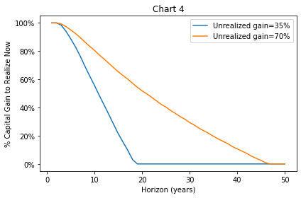
We can see that if you have a short horizon, it’s optimal to realize a high fraction of current gains – but as horizons lengthen out, you want to realize less and less. Why might this be? For a very short horizon, say just one minute, it makes sense to realize 100% of the gain right away, re-establish the position and then liquidate it after the 1 minute has elapsed.¹² Over that very, very short horizon, it’s fair to expect very little price change in the risky asset, so taking the gain now is pretty much a no-risk, no-brainer. However, as the horizon gets longer, risk enters the calculus as the relative benefit of the realization decision is tied to the risky asset price at the horizon, as illustrated in Chart 1. The risk of early realization has the general profile of being short an option: if the asset price doesn’t move much, the investor is better off taking advantage of the lower tax rate by realizing early, but if the asset price goes down or up dramatically, deferring realization will have been the better decision. A big drop in the asset price will leave the investor with a non-refundable tax loss,¹³ while a big rise in the asset price favors deferral as it allows the investor who hasn’t paid tax early to have a larger exposure to the risky asset. At the same time, the time value component of deferring paying taxes goes up with an increasing horizon. These two effects shift the balance towards deferring realization as horizon lengthens.

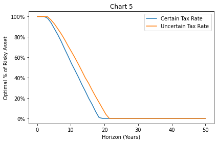
So far we have treated the future capital gains tax rate as known with certainty, but it’s easy enough to see how tax rate risk impacts the realization decision. In Chart 5, using the assumptions in our base case, we plot the optimal realization decision comparing the case where the capital gains rate increases to 50% versus the case where there’s an equal chance that it’s unchanged at 30%, goes up to 50%, or goes up to 70%. Notice that all we’ve done is introduce tax rate risk, as we’ve left the expectation of a 50% future tax rate the same in both cases. What we find is that tax rate uncertainty pushes the investor to realize more gains at every horizon up to a horizon a bit beyond 20 years, when full deferral is suggested under both sets of future tax rate assumptions. The reason we get this result is that our investor is risk-averse, and uncertainty in the future capital gains tax rate introduces risk into deferral.¹⁴

Conclusion

Making sound financial decisions under uncertainty requires finding the decision that maximizes your expected risk-adjusted wealth. Doing so often involves more than a back-of-the-envelope calculation, but the math is not terribly complex – and we’ve provided a calculator to do the heavy lifting for you. While the cases we’ve dealt with in this note have been simplified, the framework we’ve proposed is flexible enough to handle more realistic setups, including a more general, multi-period lifetime saving, spending and investment framework, and also an integration of correlations between tax rates, asset prices, inflation and interest rates. If you’re interested in building your own calculator to handle more complex or personalized cases, we’ve shared our Jupyter Notebook with the core framework, equations, and Python code.

The core points we’d like to leave you with are:

The expected-utility framework is superior to a static analysis for answering tax questions involving uncertain outcomes and produces sensible results which maximize risk-adjusted wealth. This approach can suggest partial realization as optimal, a solution that is not possible within the conventional solution.
Horizon is very important: At shorter horizons, it tends to make sense to realize some amount of gains early when capital gains tax rates are expected to rise, while deferring gains is more attractive at longer investment horizons.
Under many circumstances, the difference in risk-adjusted wealth between the optimal decision and a bad decision is great enough to warrant an investor spending some time to make a thoughtful decision. However, in the neighborhood of the optimal decision, risk-adjusted wealth differences are small, so it’s reasonable to get in the ballpark of the best decision without worrying about a high degree of precision.

In practice, most investors see themselves as having multiple horizons over which they expect to liquidate assets to fund spending, and portfolios generally have a mix of assets with different cost bases and different characteristics. This adds complexity to the analysis, but doesn’t change its basic character – making decisions that maximize expected risk-adjusted wealth is the best way to improve your expected welfare.

We encourage you to spend some time with our calculator, and please do get in touch with us if you’d like to discuss using this framework or how it might be applied to your individual circumstances and decisions.

Disclaimer:

In this note, we’ve provided a framework for thinking about tax-related investment decisions. Nothing in this note should be construed as tax advice pertaining to any individual’s specific circumstances, and your authors are not tax experts. We have simplified the problems we have discussed considerably, ignoring many important tax rules, including (but not limited to) discussions of the impact of different rates for long-term versus short-term capital gains tax, different rates at different income levels, the value of capital gains tax loss carryforwards, estate, trust and charitable considerations, and many, many more.

Technical Appendix

The capital gains tax rate τ₀ will be changing tomorrow to τ . You have some amount of homogenous unrealized gains g₀ , and you want to know whether you should realize your gains now (or more generally, what fraction should be realized), given that you also want to hold the optimal of the risky asset to horizion T , at which point you’ll realize any additional gains and pay any taxes.

We assume the risky asset S follows a GBM with mean return μ and volatility σ , and that you have CRRA utility with elasticity γ . S also pays a dividend at rate δ which is taxed at τ_d .

As usual, we want to optimize expected utility:

U(θ,κ) = 𝔼 [u P̂_T]

where:

u(w) { w^{1 – γ} – 1 1 – γ , γ ≠ 1

u(w) = ln(w), γ = 1

P̂_T = P_T – (φ⁺ + α(1 – T T_c )⁺ φ^–) τ

φ = (1 – θ – ε)g + P_Te^–κ T δ(1 – τ_d) – P₀

ε = 1 κ₀ ((κ₀ – κ)⁺ – κ₀ θ)⁺

P_T = P₀e^{(κ(μ – δ_Td) + (1 – κ)(1 – τ₁)r – ½ κ² σ²)T + κ σ Z_T}

P₀ = 1 – (θ + ε)g_τ 0

Note: ε is the amount of extra immediate gain realization (if any) additional to θ called for by rebalancing the risk asset from κ₀ to κ . α is the multiple applied to the asset value of a loss carryforward if received today, and T_c is the time after which loss carryforwards have no asset value.

Email Us

Call Us