October 16, 2017
Investment Theory
Some Clarity on Risk Parity
By Victor Haghani and James White 1
This post was first published on Bloomberg Prophets.
Google “risk parity” and you’ll see a grab bag of conflicting results: articles and posts trying to explain what it means, why it reduces stock-market volatility, why it increases stock-market volatility, why it’s less risky than a traditional portfolio, or why it’s more risky, among other things.2 We’ll try to cut through this confusion to show that risk parity and traditional portfolios are closely related in philosophy.
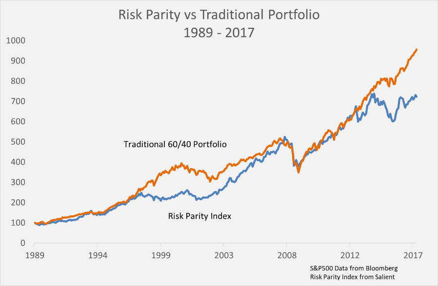
Risk parity is all about how an investor allocates risk, not capital, typically with the use of leverage and with the idea that an equal risk allocation to various asset classes increases the benefits of diversification. Risk parity and traditional portfolios are usually presented as being philosophically miles apart, and hard to compare or analyze side by side except by looking at the historical record, such as in the chart below. The problem, though, is that financial market history is limited in that it reflects only a very specific set of historical conditions and, as we know, past performance isn’t indicative of future results.
What’s an investor to think? Both types of portfolios come out of the same theory of portfolio construction, but with different sets of basic starting assumptions. The theoretical toolkit we’re talking about here is the “Optimal Expected Utility” framework applied to financial markets by Paul Samuelson and his protégé Robert Merton starting in the 1960s.3 Their work helped them both garner a Nobel Prize, and produced a set of practical tools for determining how much of one’s wealth should be allocated to different investments with the understanding that the future is uncertain. The tools are primarily based on an investment’s expected excess return, volatility, and the investor’s personal level of risk-aversion.4
The basic idea is that an investor’s utility doesn’t keep going up as investment size – and thus risk – increases, but instead there’s an optimal investment size that maximizes expected utility given one’s personal level of risk-aversion. This simple idea leads to some powerful results. With the five assumptions below, the utility toolkit tells us that the portfolio that maximizes expected utility is the one with the highest Sharpe ratio – a common measure of risk-adjusted returns5 – levered or de-levered to an optimal level of risk.
- Assumptions for Optimality of Basic Risk Parity Portfolio:
- All assets follow a random walk and are continually tradeable
- All assets have equal pair-wise correlation with each other
- All assets have equal Sharpe ratio over a long horizon6
- Unlimited leverage is available at the risk-free rate
- No fees, transactions costs, or other drags on return
To build that portfolio with uncorrelated, equal-Sharpe ratio assets, we’d hold an amount of each asset that is inversely proportional to its volatility, resulting in each asset contributing an equal amount of risk to the portfolio. This is why it’s called “risk parity” investing.7 Using some stylized risk/return assumptions, the table below shows how this works with two risky assets for an investor with a “typical” amount of risk aversion.8 The first three rows show arbitrary allocations, and the final three rows show utility-optimal allocations corresponding to the given portfolio assumptions.
| Portfolio | Stocks | Bonds | Expected Excess Return | Risk | Sharpe Ratio |
Risk-Adjusted Return |
| Stocks | 100% | 0% | 4.0% | 16.0% | 0.25 | 0.2% |
| Bonds | 0% | 100% | 1.0% | 4.0% | 0.25 | 0.8% |
| Traditional | 60% | 40% | 2.8% | 9.7% | 0.29 | 1.4% |
| Risk Parity Unlevered |
20% | 80% | 1.6% | 4.5% | 0.35 | 1.3% |
| Risk Parity Levered |
50% | 200% | 4.1% | 11.6% | 0.35 | 2.1% |
| Risk Parity + 0.6% Extra Borrow Cost | 45% | 85% | 2.5% | 8.0% | 0.31 | 1.5% |
The Merton toolkit suggests our investor would optimally want to own, via leverage, $250 of the equal-risk portfolio for every $100 of savings, resulting in the “Risk Parity Levered” portfolio in the table. The performance of this portfolio is quite a bit better on a risk-adjusted basis, 0.7 percent a year to be exact, than the traditional 60/40 stock/bond portfolio.9
We made some strong assumptions to get this result. Let’s see what happens when we loosen just one of them and assume that leverage isn’t available at the risk-free rate, but at a rate 0.6 percent higher? That cuts the risk-adjusted return of the optimal portfolio to 1.5 percent per year. This portfolio is very close, both in risk-adjusted return and Sharpe ratio, to the traditional 60/40 portfolio, making the traditional portfolio functionally optimal given the assumptions. We get the same result if we assume the investor doesn’t want to use leverage, regardless of the rate. Changing this assumption isn’t some abstract technicality: Leverage in real markets is not freely available at all times or at consistent rates, and there are many reasons an investor may choose to eschew leverage.10
The portfolios we see here represent two ends of a spectrum – but the range is surprisingly narrow. In our admittedly stylized two-asset example, only 0.7 percent per year of risk-adjusted return separates the fully-levered risk parity portfolio from the unlevered traditional one, which gives a sense for the level of fees, trading costs and extra borrowing expense a risk parity strategy could plausibly support.11 If the five assumptions above seem reasonable, risk parity portfolios may make sense for you, but if not, a more traditional portfolio may be a better fit, and is just as consistent with good finance theory.12
- Victor is the founder and CEO of Elm Partners, a HNW Robo-investment manager. James works with Elm Partners in addition to pursuing his own research and investment interests.
- There are a number of overviews of risk parity online. Here’s one: “Understanding Risk Parity”.
- 3 One of the most seminal papers is Robert C. Merton’s “Lifetime Portfolio Selection under Uncertainty: the Continuous-Time Case.” The Review of Economics and Statistics (51), 1969.
- A core result is that, for one risky asset following a random walk, the optimal investment size is where (μ – r)/(n * σ2) is the asset’s excess return, σ its volatility, and n the investor’s coefficient of risk-aversion. We often refer to this result as the “Merton Rule.”
- Sharpe Ratio is the ratio of an asset’s excess return to volatility: SR = (μ – r)/ σ)
- This is consistent with both the historical record and what many equilibrium models would predict.
- Assuming risk and volatility are interchangeable for the purposes of this discussion. For uncorrelated assets with different Sharpe ratios, the solution is to scale each proportional to Sharpe ratio and inversely proportional to risk.
- We’ll define typical here as that degree of risk aversion that would maximize expected utility by investing 100 percent of savings in a stock/bond portfolio with a 60/40 mix. With the numbers in our illustration, this implies a coefficient of risk aversion in the Merton model of 3. For readers familiar with the Kelly Criterion, this means our investor is 3 times as risk averse as a Kelly bettor. Also, typical risk parity implementations include four or more assets, including commodities and credit.
- Risk-adjusted return = Expected Return – ½ * σ2 * n , where n is the coefficient of risk aversion.
- A few reasons that come to mind: 1) real markets may not follow pure random walks but can also gap, 2) leverage may not be easily adjusted once set, 3) terms other than rate may not be attractive, or 4) whenever the investor hears the word “leverage” he or she suffers painful flashbacks.
- And they are separated by only 0.06 in terms of Sharpe ratio, although some back-tests suggest a difference of close to 0.2. As discussed in “What’s Past is Not Prologue,” we cannot rely on historical data on its own to support or reject the existence of this amount of difference in Sharpe ratio.
- The authors would like to thank Larry Hilibrand and Vlad Ragulin for their help.