February 26, 2018
Investment Theory
What Gamblers Can Teach the Buy-and-Hold Crowd
By Victor Haghani and James White 1
The ongoing attack on stock-picking waged over the past 65 years now clearly has the upper hand. Early combatants included Markowitz, Samuelson, Sharpe, Fama, and Bogle, and as testament to their success it has become part of the conventional wisdom that ordinary investors should invest primarily in highly diversified, low cost, tax efficient index funds.
It’s become almost a corollary to this view that market-timing is also a fool’s errand; investors can’t hope to beat the market by predicting if the market is going to go up or down in the next day, month or year. Authors such as Burton Malkiel, through his influential book “A Random Walk Down Wall Street”, have argued that the Efficient Market Hypothesis, and its attendant Random Walk Hypothesis, mean that investors can only expect to hurt themselves by market timing. Many financial advisers, human and robotic, follow this line, recommending that investors should choose a level of stock market investment they are comfortable with and stick to it for the long term.2
The cases against stock-picking and market-timing seem to be pointing in the same direction: an investor can’t reasonably expect to beat the market. On closer inspection though, these activities have meaningful differences. Stock picking is largely a zero-sum activity dependent on market inefficiency. What one stock picker makes relative to the market must be the loss of another with the offsetting overweight and underweight portfolio holdings. In contrast, varying one’s exposure to the market is not zero-sum and need not rely on market inefficiency, as we’ll explore further below. One investor increasing her exposure doesn’t necessarily require a reduction from another. In fact, all investors can increase or decrease their exposure at the same time, either through a change in the price of the stock market,3 or through a change in the amount of equities outstanding. Rather than being a ‘bet’ versus the market or another investor, one investor’s optimal level of market exposure is a matter of how much risk is right for that investor given her forecast of the reward and risk of the market and her personal level of risk aversion.
The investing and gambling literature has long supported the idea that investors should change their exposure as their expectations4 of return and risk change. The Merton Rule in investing and the closely related Kelly Criterion in gambling are formal models of an entirely common-sense concept: the amount of savings we should optimally expose to the favorable but uncertain gamble of investing in the stock market should vary in proportion to expected return, and in inverse proportion to risk and our level of risk aversion.5 Under this model, the proposition that investors should hold a constant market exposure requires that either the expected excess return remains constant through time, or that the risk/reward ratio stays constant.6
Let’s focus first on expected excess return. Most researchers and practitioners would tell us the expected excess return of the stock market isn’t constant. For example, Yale Professor Robert Shiller has shown that the Cyclically-Adjusted Price to Earnings (CAPE) ratio of the stock market is a decent predictor of long-term real stock market returns, as shown in the chart below.7 Note that the return data as a function of CAPE is not primarily a result of the mean-reversion of CAPE; rather it is mostly explained by the starting earnings yield of the market, much as the 10-year return on a 10-year bond is almost entirely predicted by the bond’s yield-to-maturity at the time of purchase.8 And CAPE is just one of a number of indicators that can be used to form our expectation for the future return of the stock market, without relying on historical averages or reversion to a “fair” or average level.9
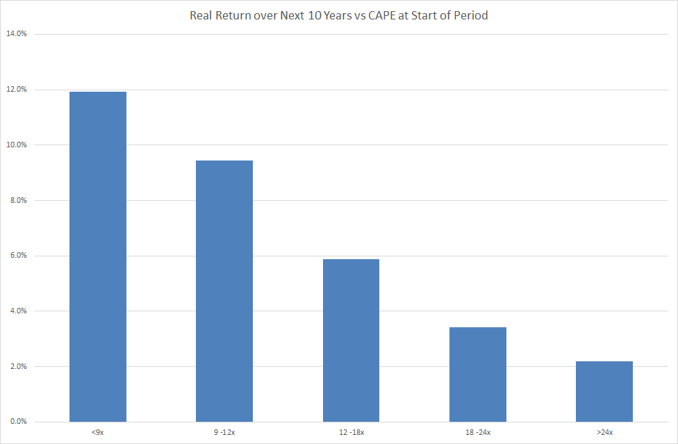
Ask yourself if you would have expected the US stock market to deliver the same long-term real return starting in 1985 when the US stock market CAPE was 10x as what it would deliver from 1965 when the CAPE was 23x?10 If you agree the lower CAPE in 1985 predicted higher expected real returns than the higher CAPE prevailing in 1965, then ex-ante, all else equal, you would have wanted a greater equity exposure in 1985 vs. 1965.11 And indeed your expectation would have been correct, as over the subsequent 30 years the real return of the US stock market was 8.2% from 1985 but only 4.2% from 1965.12
Believing that the expected excess return of the stock market changes over time is not at odds with a belief in market efficiency. Just like the price of milk and eggs, the expected aggregate real returns available in the market are a function of supply and demand, in particular the supply of investments and the demand from savers. As this supply/demand dynamic changes over time, so too do expected market returns, even in the perfectly efficient markets imagined by financial theorists.
Next, do we think it’s reasonable to assume the stock market’s risk/reward ratio stays constant? It seems plausible that an increase in expected return would be accompanied by, or maybe even caused by, an increase in expected risk.13 But while it is plausible it is not required, nor do we think it likely that such changes in risk exactly offset changes in expected return to leave the risk/reward ratio constant. For example, while expected returns were very different from the starting points of 1965 and 1985, as detailed above, the realized stock market risk over the two ensuing 30-year periods was virtually the same. Indeed, there is no theoretical reason to presume this ratio wouldn’t change over time. In fact, theory tells us that, for a given amount of savings, if there was a net issuance of new equity we should expect returns to go up without a material change to risk.
Critics of variable investment sizing point to the historical record to show that an investor would have been better off keeping a fixed fraction of their portfolio invested in equities rather than varying it based on a forward-looking, expected return predictor.14 In the Appendix, we show that a more careful look at the past 118 years of U.S. experience does not support that claim. By basing our analysis on the Merton Rule, we also counter the argument that back-tests of variable asset allocation require knowing the CAPE average in advance. We have put this analysis into the Appendix because we believe that expectations-driven sizing stands on its own logic, and that the limited US stock market history, while supportive, should not be taken as the primary reason to follow this approach.
When we look back to assess whether we’ve been well-served by following an expectations-driven approach, we must be careful to view outcomes not solely on how much we have grown our wealth, but also take account of how much risk we have taken along the way. To illustrate what we mean, imagine you are presented with the opportunity to bet on a coin that has a 70% chance of landing heads. You determine you want to bet 20% of your wealth on each flip.15 Then you are told that this coin is being replaced with a coin that has a 60% chance of landing heads. You now change your betting fraction to only bet 10% of your wealth on each flip, which is the rational, Kelly-consistent thing to do. In the next 100 flips, 60 come up heads and 40 come up tails, exactly what you expected for a 60/40 coin. You calculate that if you had still been betting 20% of your wealth on each bet, you’d have more wealth. Did you make the wrong decision to reduce your betting size from 20% to 10% of your wealth? We suggest you did not, because there was a higher chance of a worse outcome, and you properly accounted for that risk by reducing your bet size accordingly. The appropriate risk-adjusted measure of return (as described in the Appendix) would show just that.
Conclusion
It’s time to dispense with the pejorative and fuzzy term “market-timing” in favor of a more precise and neutral description for the kind of systematic, proportional change in investment sizing embodied by rules such as the Merton Rule and Kelly Criterion. We propose “expectation-driven sizing”, though we admit that doesn’t quite roll off the tongue.16
We’ve tried to show that variable, expectation-driven asset allocation is both theoretically sound and intuitively appealing. When the market offers lower expected returns, all else equal, it’s both good theory and good sense to own less of it. There’s a fundamental flaw in the prevailing conventional approach, in which the investor decides how much risk to take based solely on whether her individual level of risk aversion is above or below average, without factoring in how much she’s earning to take that risk. It would be like deciding to bet the same amount on a biased coin whether it’s 60/40 or 70/30 in your favor.
The goal of expectation-driven sizing is not for investors to beat the market, but rather to make the most of what the market is offering at each point in time, on a risk-adjusted basis. Somewhere along the road, this common-sense investing idea became confounded with the zero-sum proposition of trying to beat the market through stock-picking or short-term market speculation.17 It’s also true that “market-timing” has acquired a bad reputation in that that many investors have instead shown a tendency to vary their exposure to the market in an ad hoc, non-systematic manner, with bad results. Indeed, we agree it would be better to keep to a fixed exposure than to chase returns by varying one’s exposure based on a simple extrapolation of recent returns, or to put one’s faith in rapid reversion to some subjective assessment of fair value.
Bottom line: Investors should continue to employ low-cost, tax-efficient index funds and ETFs as the building blocks of their portfolios, and they should not be afraid to vary their exposure to the market in a disciplined fashion based on its expected attractiveness, which at Elm Partners is exactly what we mean by Active Index Investing®.
Appendix: A Closer Look at Static vs Expectations-Driven Sizing through 118 years of US Equity Market Experience
While the analysis below finds that an expectations-driven sizing of exposure to the U.S. equity market delivered superior risk-adjusted returns to a hypothetical investor under a given set of assumptions, we must stress that the past 118-year historical record of one stock market isn’t enough data to reach a statistically significant conclusion.
The table below compares the inflation-adjusted return an investor would have earned following:
1) a static, constant allocation of 65% in the S&P500 and 35% in US T-bills, or,
2) a return-driven, variable allocation between the S&P500 index and US T-bills, using the Merton rule for sizing.
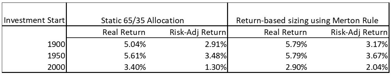
Notice that expectation-driven sizing produces higher risk-adjusted real returns over the three periods considered in the table (see assumptions box below for how we calculate risk-adjusted returns). Of note is the most recent 18-year period starting with the year 2000, to which the critic of variable sizing might call our attention. Over this period, a static 65% allocation to equities produced a higher realized return than what an investor would have earned with the smaller allocation to equities called for by the Merton Rule. The reason for this is simple: over the past 18 years, CAPE has averaged 25.8x which indicated a low long-term expected excess return for equities, and hence it would have been sensible for a risk-averse investor to have a relatively small exposure to equities. Indeed, it transpired that the real return of US equities over the past 18 years was a relatively meager 4.79%. So, our investor who held less equities was justified ex-ante and ex-post in holding less equities, but we can only see this if we compare the risk-adjusted real return earned by the two strategies, not their gross returns. It is only by explicitly taking risk into account that we can see clearly that even though the investor who held less equities wound up with less wealth today, he was better off after taking risk into account, enjoying a real risk-adjusted return of 2.04% versus 1.30%.
Assumptions:
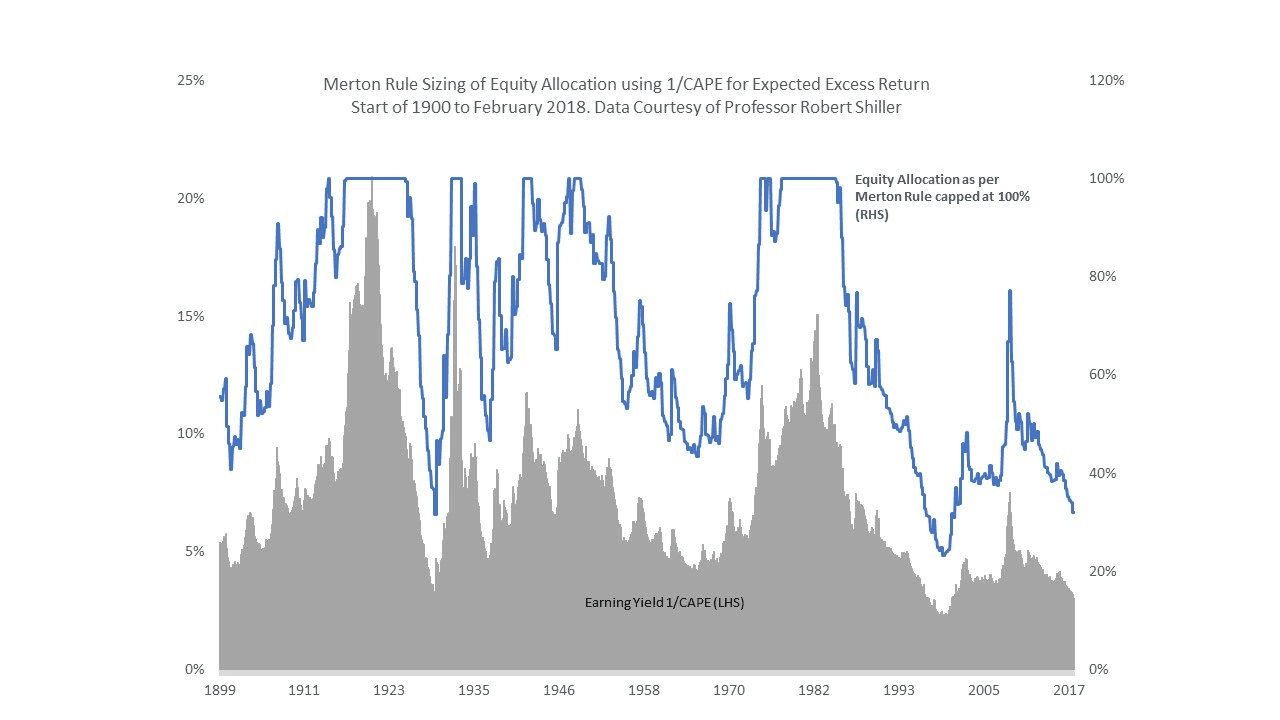
Data from Professor Robert Shiller’s website, from the start of 1900 to February 2018. Quarterly rebalancing using Merton Rule, with 1/CAPE for expected excess return on equities, hypothetical investor with CRRA utility with coefficient of risk aversion, η = 3 , assuming equity market volatility throughout of 18% pa, equity market follows geometric Brownian motion, 0 leverage allowed which was binding at different times (see chart above). For example, at CAPE = 16 , optimal equity allocation is 64%.
Risk-adjusted returns calculated by subtracting η(ασ)22, where α is fraction of wealth invested in the stock market, σ = 18% , and η = 3 . We used 1/CAPE for the expected excess return of equities as we did not have a long-term forward-looking estimate of the real rate on the risk-free asset, and we feel that 1/CAPE is an under-estimate of long-term real returns of equities of about 1%, which we think would have been close to the long-term expected real rate since 1900.
- Victor is the Founder and CIO of Elm Partners, and James is Elm’s CEO. Past returns are not indicative of future performance. This not is not an offer or solicitation to invest.
Thank you to Larry Hilibrand, Antti Ilmanen, Spencer Jakab, Arjun Krishnamachar, Bruce Lafranchi, Andy Morton, Vlad Ragulin, Jeff Rosenbluth and Rich Dewey for their very helpful comments and suggestions. A working draft of this note was discussed by John Authers in this Financial Times article.
- An exception to the strict rule allowed for reducing the allocation to equities in old age.
- As we discuss here.
- Throughout this note we use “expectation” and “expected” in the common-language sense, not in the sense of mathematical expectation.
- The Kelly Criterion is a gambling rule for sizing favorable bets proposed in 1956 by John Kelly, a mathematician at Bell Labs. Optimal Fraction of Bankroll to Invest = p – q = 2p – 1 , where p is the probability of winning and q of losing. In other words, for a bet where the bettor can win or lose equal amounts, the optimal percent of your bankroll to bet is equal to your “edge,” defined as the extent to which the probability of winning is in your favor. The more favorable the probability of winning, the more you should bet. The Kelly Criterion is a special case of a more general rule for investing derived by Robert Merton and published a few years later in 1969.
The Merton Rule: Optimal Fraction of Wealth to Invest = μ σ2 η
where μ is expected excess return, σ is risk expressed as Standard Deviation, and η is the degree of risk aversion held by the investor in question, where η = 1 represents the same degree of risk-aversion as embodied in the Kelly Criterion (a “Kelly bettor”), and η = 2 describes an investor who is twice as risk averse as a Kelly bettor.
- In this context, risk means variance. There is another possibility, which we view as more complex and less realistic than needed to make it into the body of this note. It is that somehow the whole ratio of the Merton rule stays constant, so that expected return, expected risk and the investor’s risk aversion all change in such a way as to keep the optimal fraction of wealth to invest constant. We believe that an investor’s level of risk aversion can be thought of as roughly constant through time.
- See Campbell, John Y., and Robert J. Shiller, “Stock Prices, Earnings, and Expected Dividends,” Journal of Finance, 43(3): 661-76, July 1988, and Robert J. Shiller, “Price Earnings Ratios as Forecasters of Returns: The Stock Market Outlook in 1996” (21 July 1996).
- For a more in-depth treatment of where CAPE’s predictive power comes from, see: “Market Multiple Mean-Reversion: Red Light or Red Herring?”
- At Elm Partners, we form our expectations of equity market returns from a combination of CAPE and momentum based on a one-year moving average.
- The dividend yield in 1965 and 1985 was respectively 2.8% and 4.3%.
- Assuming your long-term estimate for the risk of the stock market was the same, which we’ll discuss more shortly.
- It is interesting that few investors would determine the 30-year expected return on a 30-year inflation-linked bond by calculating the past 100 years of average returns on 30-year inflation-linked bonds—they would just look at the real yield the bond was being offered at today. Yet there are many investors who determine the expected long-term real return of the stock market based on the past 100 years of stock market return.
- Unfortunately, it’s difficult to test this empirically, as while we can observe realized volatility as a proxy for current risk, we cannot directly observe expectations of long-term market risk. If there were observables linked to market prices, it would be difficult to disentangle the true expectation from the risk or insurance premium built into those prices. It is also not possible to derive expectations of risk from expected cash flows in the way we do when determining long-term expected returns for equities or bonds.
- For a more in-depth treatment see: C. Asness, A. Ilmanen, T. Maloney, Market Timing: Sin a Little, Resolving the Valuation Timing Puzzle, Journal Of Investment Management, Vol. 15, No. 3, (2017), pp. 23–40, here.
- We’re assuming you’re twice as risk-averse as a Kelly bettor.
- Please send us your suggestions for something more catchy!
- While typically experiencing high frictions for the privilege.