December 14, 2021
Investment Theory
For Crypto Whales: When Less is More
By Victor Haghani and James White 1
In general, the more optimistic we are on the prospects of an investment, the more of it we’ll want to own. However, at extreme levels of bullishness, the normal relationship can be turned on its head and it can make sense to own less of an asset the more we like it. It’s hard to think of everyday examples that work like this, so this poses something of a puzzle. It’s a problem which gets little attention in mainstream finance, because we rarely witness high enough forecasts of investment quality to observe this effect in the wild.2 We can thank the digital-asset revolution and its band of optimistic crypto-asset enthusiasts for bringing this problem into focus, which also gives us some valuable insights that apply in other domains of financial decision-making.
Risk-Aversion
We’ll assume a representative Investor with a relatively moderate level of risk-aversion.3 For those familiar with the Kelly Criterion, we’re assuming an investor with twice the risk-aversion of a Kelly Bettor.4 Many individuals find that while “full” Kelly may be appropriate for cash management in blackjack or poker, it calls for too much risk when applied to total wealth. In gambling circles, our Base-Case investor would be called a “half-Kelly bettor”, and would find himself in the company of quite a few famous investors who also size their risks in line with this level of risk-aversion. More concretely, such an investor would be indifferent to a 50/50 coin flip which could increase his wealth by 50% or decrease it by 25%.5
Crypto Risk and Return
It is hard to know how to accurately model the price behavior of digital assets, but most would agree that they do not follow the continuous Geometric Brownian motion of finance textbooks, and their returns are far from being well-described by the standard Normal distribution. Financial assets in general (and digital assets in particular) experience price jumps and fat tails, and their variability and expected returns are difficult to estimate and can change dramatically over time. Additionally in the case of digital assets, many investors recognize some risk of losing their investment through hacking, hard forks, loss of private keys, etc – more like seeing one’s house burn down rather than experiencing a bad run in the market. To cut through all the uncertainty of crypto return distributions, we’re going to radically simplify and assume that to some chosen horizon there’s a 50% chance the asset goes to 0, and a 50% chance it goes up by a factor of P, the “payoff ratio”.
A Puzzling Result
The chart below shows the optimal amount our Investor should allocate given a range of payoff ratios.6 As we increase the payoff ratio from 1:1 to 2048:1, the expected return and risk of the asset goes up – and crucially, the ratio of return-to-risk, the Sharpe Ratio7, is also going up. That’s what we mean when we say that the quality of the investment is getting better and better.
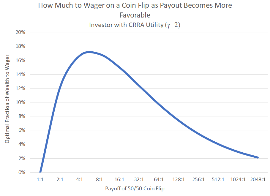
When the expected payoff ratio is between 4:1 and 8:1, the optimal allocation reaches its peak at about 17%. Then – and this is the whole point of this note – at higher payoff ratios, the optimal bet size declines. For very optimistic investors (and believe us, there are some really optimistic ones out there8), an allocation potentially well under 10% may be optimal.
Explaining the Hump
An intuitive explanation for this hump is this:
- It starts at zero: At the 1:1 ratio at the far left of the chart, since the upside and downside are equally likely and equal in size, the optimal allocation starts at zero since the investor shouldn’t take risk without some expected reward.
- Then it goes up: As we increase the payoff ratio by moving to the right, the investment opportunity warrants some allocation of capital.
- Then it eventually goes back down to zero again: At some point (rarely seen in practice), when an asset is sufficiently great, holding even a small amount of it will make us fabulously rich in the good outcome – so there’s no reason to hold a ton of it and risk the bad outcome on a large fraction of wealth. Put another way, since we can get as much cake as we can ever eat for a pittance, why spend a penny more?! This effect takes the optimal allocation back down again towards zero, giving us the hump shape.
While the circumstances that give us this result are something of an oddity, a closer look at what’s going on gives us insights about wealth and risk that are more broadly applicable.
A Different Perspective on Wealth and Risk
Normally, we think of our financial wealth as the sum of the current market values of the assets we own.9 This works well enough in most circumstances, but when an investor feels he has come across an outstanding gem of an investment, using the market price for that asset rather than a value that reflects the higher intrinsic risk-adjusted value can lead to suboptimal decision-making. Encountering an asset – a digital asset, in this case – that the investor believes has a 50/50 chance of delivering a 100:1 payoff ratio makes him effectively wealthier than a standard mark-to-market accounting treatment would indicate. If he really believes in the attractiveness of the investment, he would need a substantial compensating payment to forego investing in it. We use the term Certainty-Equivalent Wealth to refer to the level of wealth that he would be equally happy to possess with absolute certainty instead of his current wealth plus the opportunity to invest in the highly-attractive asset.
To illustrate, say our investor decides to invest 17% of his wealth in a crypto-asset that has a 50/50 chance of going up eight-fold or down to zero. The expected return of the asset is 300%, and the investor’s expected wealth is 150% higher than his starting wealth – but his Certainty-Equivalent Wealth is that level of wealth that he’d be just as happy having for sure but without the ability to buy the attractive crypto-asset. Using our Base-Case investor’s preferences, we can calculate that his Certainty-Equivalent Wealth should be about 125% of starting wealth.
We now turn to the question of risk: how much risk is the investor taking in the above illustration? Normally, one might say that his downside is losing 17% of starting wealth, and that is his risk – but that ignores that his “true” wealth, his Certainty-Equivalent Wealth, is 125% of his nominal starting wealth because he bought this great investment that sports a 300% expected return. If that’s his relevant starting wealth, now we see that his downside is much higher, at 34% (the loss from his wealth going from 1.25 to 0.83) if the asset’s downside case is realized. Just like we’d expect, as the investment gets more attractive the investor is indeed taking more downside risk, measured against his Certainty-Equivalent Wealth.
Conclusion
“All models are wrong, but some are useful.”
– George E.P. Box
The assumptions we’ve made in this analysis have been chosen for simplicity and illustration. In particular, we recognize that modeling outcomes of digital assets in a binary manner is not realistic, though it does capture a certain kind of view that digital assets will either go to the moon or fade away. But the general effect we describe, that the optimal holding of an asset at some point goes down as its attractiveness goes up, holds over a pretty broad range of assumptions about distributions of outcomes and investor risk preferences.10
Moreover, the insight that we should view our base wealth as inclusive of the value provided by attractive investment opportunities is important and applies in other situations. For example, a hedge fund or private equity manager might be prone to over-investing in the fund he manages if he underestimates the value and risk associated with his ownership interest in his fund management business.
If you think you have an investment opportunity that might benefit from this kind of analysis, we’d love to discuss it with you.
Further Reading and References
- Black, Fischer. “Noise”. Journal of Finance (1986).
- Haghani, Victor and James White. “Measuring the Fabric of Felicity”. SSRN (2018).
- Kelly, John, L. “A New Interpretation of Information Rate”. Bell System Technical Journal (1956).
- Merton, Robert, C. “Lifetime Portfolio Selection under Uncertainty: the Continuous-Time Case”. The Review of Economics and Statistics (1969).
- Thorp, Edward, O. “Fortune’s Formula: The Game of Blackjack”. American Mathematical Society (1961).
- This not is not an offer or solicitation to invest, nor should this be construed in any way as tax advice. Our thanks to Steve Mobbs for his input on this note. Past returns are not indicative of future performance.
- For example, in his 1986 Presidential address to the AFA titled “Noise”, Fischer Black stated:“…We might define an efficient market as one in which price is within a factor of 2 of value, i.e., the price is more than half of value and less than twice value…By this definition, I think almost all markets are efficient almost all of the time…”
- As per a survey we conducted in 2018 of thirty financially sophisticated investors and described in “Measuring the Fabric of Felicity”, we assume our Base-Case investor is in the bottom quartile of risk-aversion.
- We assume the investor exhibits Constant Relative Risk Aversion (CRRA), with a coefficient of risk aversion, γ , of 2. CRRA Utility can be written as:
U(W) = (1 – W(1 – γ)) / (γ – 1) for γ <> 1 , and
U(W) = ln(W) for γ = 1 . γ = 1 gives us the Kelly Criterion, and γ = 2 is referred to as “half-Kelly”. - Feel free to get in touch with us if you’d like some guidance on calibrating your personal level of risk-aversion.
- The optimal allocation k* is that which maximizes the investor’s Expected Utility. Given a payoff ratio P upside probability π and Constant Relative Risk-Aversion coefficient g ,
k* = (P – π P)1/g – π1 / g (P – π P)1 / g + π1 / g PWe are assuming this is the only investment opportunity available.
- Technically, the ratio of expected return to standard deviation, assuming a 0 risk-free rate.
- One example of a highly optimistic investor is Michael Saylor, CEO and founder of MicroStrategy (MSTR), an owner of several billion dollars of digital-assets. On August 18th, 2021, he stated here that he expected Bitcoin to become “a $100 Trillion asset.” Given the price at which Bitcoin was trading at the time of his statement, it implied a hundred-and-twenty-fold increase in the price of Bitcoin.
- Investors in private, illiquid assets often think of them at their cost basis, or somewhere between cost and an estimate of fair market value.
- But not all whales are of the humpback variety. Two notable cases where it may not hold are: 1) if the asset follows a continuous random walk and the investor can rebalance his portfolio continuously without frictions, or 2) for an investor with risk-tolerance equal to or greater than a full Kelly bettor, i.e. whose utility function is at least as risk-tolerant as U(W) = ln(W) .