By Victor Haghani and James White ¹

“There is nothing either good or bad, but thinking makes it so.”
  – William Shakespeare, Hamlet Act II (1602).

If you had put $100,000 of your savings into Bitcoin at the end of 2020 and are still HODLring (crypto-nese for “holding on for dear life”) those coins today, you’d be down 20% on your investment given its drop in price from $25,000 to $20,000 (as of July 5th).

If going long was no good, how about going short? An investor who put $100,000 into a crypto-brokerage account to short $100,000 of Bitcoin, with no further trading, would have been wiped out just a few months later in mid-February 2021 when Bitcoin more than doubled. This kind of shorting is effectively a form of automatic doubling down, since as the value of the asset goes up, the value of the capital supporting it goes down, causing the short position to get bigger and bigger (quickly) relative to capital.² So, while “buy and hold” is a real strategy, “sell and hold” isn’t generally workable in practice. Instead, the short position that most closely represents the opposite of the buy-and-hold long position can be thought of as funding an account with that same $100,000 and then establishing and managing the short position so that at all times the size of the short is equal to the account’s liquidation value.

How would this managed short have done since the end of 2020? While avoiding total wipeout, an investor shorting Bitcoin in this way would still have lost 50%. That’s right…over the past 18 months, you’d be down 20% from a 100% Bitcoin long position, and down 50% from the opposite managed short.³ Naturally, this seems strange and unfortunate! To help understand why it’s the case, we’re going to see if there’s some other constant proportion of capital – other than 100% long or 100% short – that the investor could have maintained, with regular rebalancing, which would have turned a profit.

We could simply search over all possible constant proportions to see which gave the best result over this period, but before we do that, let’s reason from first principles to figure out what we should expect to find. We tend to think about the quality of an investment by calculating its historical Sharpe Ratio, which takes the realized return of an asset in excess of the risk-free rate and divides it by the asset’s risk. Over this period, Bitcoin’s realized Sharpe Ratio, calculated from average daily returns, was +0.2. (for a deeper dive into how Bitcoin could have had a negative return of 20% but a positive Sharpe Ratio, see this footnote ➚)⁴ This suggests that Bitcoin was a fair, but not great, investment over this period – by comparison, broad equity markets have expected Sharpe Ratios of around 0.3. The optimal allocation to not-so-great, but very risky investments should be fairly small, so if there’s a capital proportion that’s profitable at all, we’d expect it to be fairly small too.

And indeed, this is exactly what we find, as indicated in the chart below.

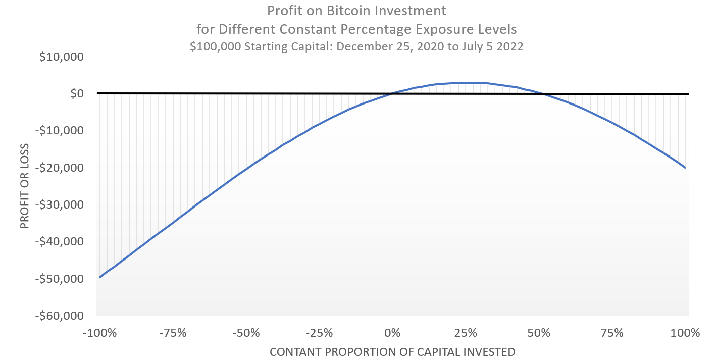
The maximum profit of $3,000 was realized for an investor who kept a constant 25% of capital in Bitcoin over the whole period.⁵ In fact, any positive proportional investment up to about 50% would have resulted in a profit.⁶ However, you don’t make twice the profit from taking twice the exposure; in fact, at 50% exposure, the profit is zero, rather than two times $3,000. Note that this is not a buy-and-hold strategy; to maintain a constant proportion of capital in an asset, regular rebalancing is required.⁷

We can also see that there are not any constant proportions generating a profit from both the long and short sides. You can lose money from a wide range of symmetric longs and shorts, but the only way to make money was to have constant long exposure in the range 0% to 50%. Put another way, you have to both correctly judge the quality of the investment, and then size your investment consistently with that quality, and getting either materially wrong will generally result in losses.

There are a few things we can take away from this mini case study:

1. These ideas are not specific to Bitcoin. We chose Bitcoin to illustrate them because they are easiest to see for highly volatile assets, and there are few assets that have been more volatile.
2. We can’t say that an investment is good or bad without considering how we will manage its sizing over time: sizing is as important as evaluating an investment’s expected risk and return.
3. While there are an infinite set of investment strategies involving a given asset,⁸ we can learn a lot from focusing on the simplest strategy: Constant Proportion investing.
4. Among Constant Proportion investment strategies, there will be a range of investment sizes that will be profitable, with sizing above and below that rapidly becoming increasingly unprofitable. And the range of profitable sizes is strongly related to the quality of the investment.
5. For a given investment, the realistic strategies which turn a profit are typically quite a small subset of the infinite number of total strategies to choose from.

1. This not is not an offer or solicitation to invest, nor should this be construed in any way as tax advice. Past returns are not indicative of future performance.
   
2. For example, if Bitcoin goes up 50%, the size of the position relative to the amount of capital supporting it would have moved from 1:1 to 3:1. Such an approach requires an unlimited amount of capital, which is an amount few real-world investors have access to. A leveraged long position requires the same sort of position management, since as the asset goes down, capital goes down faster, and the investor will need to sell some of the asset to keep the leverage ratio constant.
   
3. You can read more about why this is the case in George Costanza At It Again: The Leveraged ETF Episode (2020). Throughout, we assume daily rebalancing, no transactions costs, no borrow fees and a zero risk-free rate. All data from Yahoo Finance.
   
4. The reason the Sharpe Ratio was positive even though the Compound return over the period was negative is because Sharpe Ratio is computed using the Arithmetic average daily return of Bitcoin over the period, which for a risky asset will always be higher than the Compound, or Geometric average, return. Under some stylized assumptions, the difference between the Compound Return and the Arithmetic Return of a risky asset is equal to one-half of the variance of returns, a quantity known as “variance drag.”
   For Bitcoin over this period, the variance drag was about 30% per annum (30% = 0.5 * 0.77² )! The Arithmetic Return was not sufficiently positive to offset the 30% variance drag, and so the Geometric Return was negative, but it’s the Arithmetic Return that ultimately determines the quality of a regularly rebalanced investment opportunity. Another perspective is to say that Bitcoin’s realized Sharpe Ratio would be positive as long as it’s Compound Return was better than -30% pa, given its realized volatility.
   For a simple example of variance drag, consider an asset that goes up and down 10% each day for 10 days. The average daily return is 0, because it went up 10% an equal number of times as it went down 10% – but the Compound return will be negative because every time it goes up 10% and then down 10%, the asset winds up 1% lower than where it started, and so the Compound return will be negative. That’s the effect of volatility, and boy has Bitcoin been volatile!
   
5. Readers familiar with the bet-sizing literature will recognize that the 25% proportion of capital corresponds to the Kelly Criterion, which over many bets– and here we have 557 daily bets– gives the highest end wealth. The Kelly calculation takes the Sharpe Ratio of 0.2 and divides it by the standard deviation of returns of about 80%, to arrive at a bet size of 0.2 / 0.8 = 25% .
   
6. Note that we will not find cases where one can find long and short fractions that would both make money, i.e. the range of profitable proportional sizing will always start at 0 and either go positive or negative from there.
   
7. Over this period, it didn’t make a material difference if you rebalance daily, weekly, or monthly. The Sharpe Ratios based on weekly and monthly returns were 0.21 and 0.23.
   
8. For example, strategies involving buying or selling puts or calls, or other kinds of dynamic scaling strategies.