By Victor Haghani and James White ¹

“The key issue in investments is estimating expected return.”
  – Fischer Black

Introduction

You’re probably familiar, at least in passing, with the ‘convexity’ of long-term bonds – i.e. that yields dropping 1% produce a bigger price move than yields rising 1%. A significant amount of brainpower has gone into understanding all the ramifications of this convexity in the fixed income markets, and the various issues and opportunities that arise are now very well understood. Equities, on the other hand, aren’t typically regarded as convex instruments.² We tend to think of equities directly in terms of their price, rather than their ‘yield’ as we do with bonds, and often think primarily about their annual return, which moves lockstep with price. But, as we discuss below, equities do have important convexity properties, and they tie into two themes we think deserve more attention: how investors think about long-term returns, and how to properly size portfolios and investments. Our story of how equity convexity, return forecasts, and investment sizing all tie together starts in the late 1960s with a remarkable result from Robert C. Merton.

The Merton Rule

A typical first step in building an investment portfolio is to forecast long-term returns, and identify the basket of investments with the most attractive return relative to their risk.³ With this accomplished, we still need to decide what percentage of our wealth to invest in that basket. In 1969, as part of his PhD dissertation under the guidance of Paul Samuelson, a 25-year old Robert C. Merton gave us an elegant and powerful rule for making that decision. Subject to a few important assumptions, the rule is simple and exact, and its simplicity and intuitive appeal make it a valuable rule of thumb. It brings together the three main variables that we would expect to be critical to the sizing decision: the basket’s expected risk and return, and the investor’s personal degree of risk aversion. Remarkably given its usefulness and beauty, this rule does not have a widely-agreed moniker; we hope we won’t cause any offense if we call it the ‘Merton Rule’: ⁴

Optimal Wealth Fraction to Invest = μ – r nσ² = Sharpe Ratio nσ

where µ − r is the basket’s expected real return,⁵ σ its annual volatility, and n is the investor’s degree of risk-aversion.⁶ To illustrate, if your estimated expected real return of your basket is 4% and its risk (standard deviation) is 16%, and your level of risk aversion is n = 3 , then the formula says the optimal fraction of your wealth to invest in the basket is 52%:   4% (3)(16%)²

While you may not have heard of the Merton Rule, you might well have come across the Kelly Criterion,⁷ which can be thought of as a special case of the Merton Rule where n = 1 and the asset can only take two discreet future values, like a coin flip.⁸ The Merton Rule and Kelly Criterion are closely related, but they were developed independently – the Kelly Criterion in the context of gambling, and the Merton Rule in the context of investment-portfolio decision making under uncertainty.

Now we’d like to point out an important aspect of the Merton Rule which is central to the purpose of this note. Owing to its derivation, the input real return µ − r must be the forecast arithmetic mean of future returns. This is an important detail that can have a sizable impact on the Merton Rule’s result, so it’s worth quickly exploring the definition of the Arithmetic Mean return, and its relation to the other widely used return metric, the Geometric Mean return.

Arithmetic vs. Geometric Mean Return and Convexity Return

The Arithmetic Mean of a sequence of rates is the simple average of those rates. In contrast, the Geometric Mean return is the single rate which, when compounded, produces the same outcome as earning that sequence of rates period by period.

The Arithmetic Mean return (AM) is always greater than or equal to the Geometric Mean return (GM), and there is a simple formula that’s a good approximation for their difference:

AM – GM ~ 1 2 σ²

where σ is the standard deviation of the sequence of rates in question. We call this difference between the arithmetic and geometric mean returns the ‘Convexity Return’, as the difference fundamentally arises from the non-linear (convex) relationship between investment value and compound rate of return,⁹ or more prosaically, that equities can go up a lot but cannot go down by more than 100%.

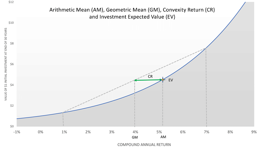
The chart above illustrates this non-linear relationship. We show an approximation of the Expected Value of the investment by averaging the better-than-expected and worse-than-expected outcomes of 1% and 7% compound returns. The Convexity Return of about 1.3% in this case is the difference between the Geometric Mean (GM) return of 4% and the Arithmetic Mean (AM) return of about 5.3% that corresponds to the Expected Value (EV) of the investment.

As you can see, the Convexity Return can be significant. The 1.3% Convexity Return we get for equities assuming 16% annual volatility is meaningful. Although the issue of arithmetic or geometric mean return may seem like a technical detail, it represents an amount of return we wouldn’t ignore or “sweep under the rug” in any other context.

To get accurate results from the Merton Rule, it’s important we’re very clear about exactly what type of mean excess return we’re forecasting, and what that forecast really means.¹⁰ When the Merton Rule was formulated in the late 60s, we suspect most academics and practitioners looked primarily to historical returns to feed their future long-term return forecasts – and in this context assuming the forecast is an arithmetic mean makes perfect sense, as taking a simple average is a natural thing to do with a series of historical return data. Now however, people use a variety of methods to generate forecasts of future returns. This got us wondering whether most people today, when they’re forecasting expected long-term returns, think of that forecast (explicitly or implicitly) as a forecast of the arithmetic or geometric mean. So, we did a survey.¹¹

The Survey

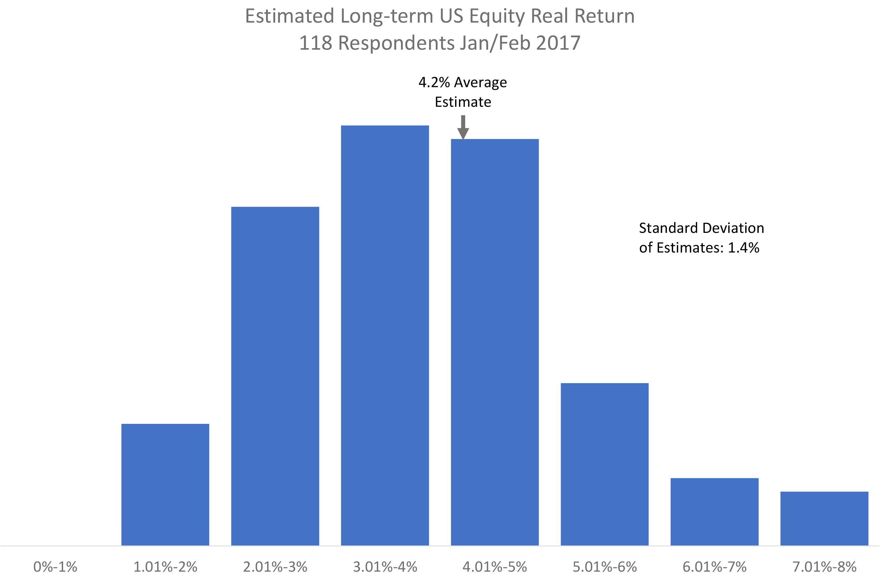Seeking the proverbial ‘wisdom of the crowd,’ at the start of 2017 we asked 118 experienced finance professionals (average age about 55), who were frequent readers of Elm’s blog posts, three questions about their views of the long-term return distribution of the US stock market via an online survey. The questions, and answers from our 118 respondents, are:

1. What is your estimate of the investment return you would earn, expressed as an annual return above inflation, on a broad US equity market index fund starting today, and holding for 30 years, reinvesting all dividends, and ignoring taxes? 4.2% as in the histogram.
2. You chose x% in Q1. At x% for 30 years, $1mm would grow into $1mm ∗ (1 + x%)³⁰ in inflation-adjusted dollars. Do you agree that there’s a roughly 50% chance that your investment turns out better than this? 83% agreed.
3. Still within the context of an investment in the broad US equity market: Which do you agree with more?
1. Over a 30-year horizon for your equity investment, realizing an outcome double your estimated investment value or half your estimated investment value are about equally likely. 77% agreed.
2. Over a 30 year horizon for your equity investment, realizing an outcome double your estimated investment value or losing all your money are about equally likely. 23% agreed.

Interpretation of Survey Results

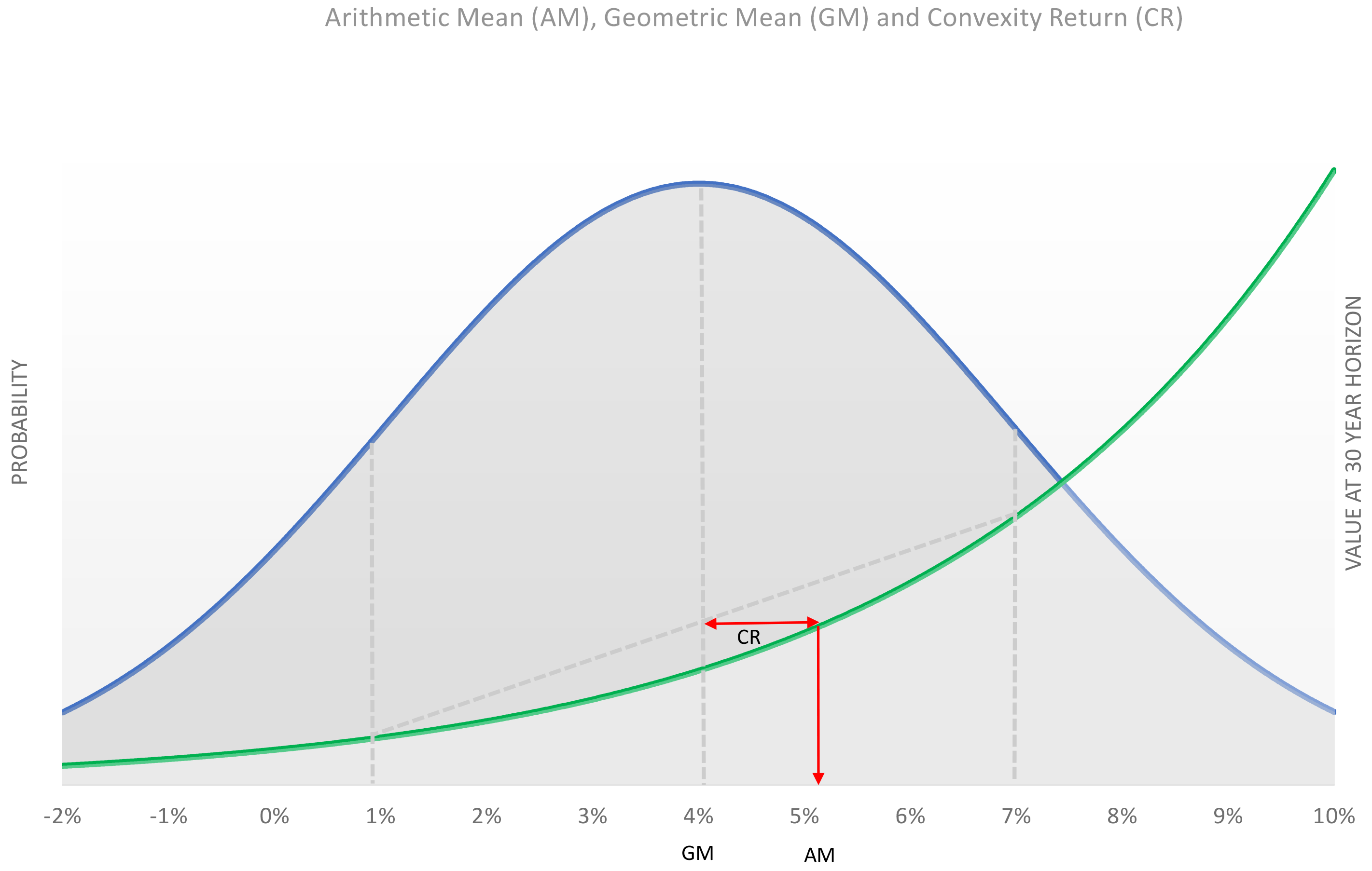What we learned from this survey was far more interesting than that the average real return estimate of our respondents was 4.2%. The chart shown to the right of a normal distribution represents more-or-less how the typical respondent would see future stock market rate-of-return outcomes.¹² We have centered the distribution at the rough average of our respondents estimates, 4% real return, to reflect the view of the 83% of our respondents who described their estimate as lying at the 50% point (median) in the distribution of outcomes.¹³ The chart also is drawn to reflect the belief of 77% of our respondents that there was about an equal chance of the investment doubling or halving versus the central outcome.¹⁴

That 83% of respondents saw their estimate as the median return is highly significant, because for a log-normally distributed asset the median return is equal to the geometric mean return. The arithmetic mean return is much higher than the median in this case; for an asset with 16% volatility, there is only a 33% chance of exceeding the arithmetic mean.

We acknowledge that, by necessity, the survey was both brief and somewhat indirect. But we conclude the results support a hypothesis that most investors are forecasting a geometric mean return, not an arithmetic mean.

Adapting the Merton Rule, with Big Impact on Optimal Allocation

But now we have a problem – the Merton Rule wants an arithmetic mean, but most forecasters are estimating a geometric mean. What to do?

Simple: to use the Merton Rule in a way consistent with how most survey respondents are estimating returns, we just need to add the Convexity Return to respondents’ return estimate. When we do this, we arrive at a ‘Modified’ Merton Rule:

Modified Merton Rule = (μ + ½σ²) – r nσ² = Sharpe Ratio nσ + 1 2n

The modification is quite intuitive.¹⁵ We simply add the Convexity Return (½σ² ) to the return estimate in the numerator. So for our typical respondent, he should set µ − r equal to his 4% excess return estimate plus 1.28% for the Convexity Return, instead of just putting in 4% as might seem natural in using the out-of-the-box Merton rule. To illustrate, using the same numbers as we did in Section 2, the modified Merton rule suggests an optimal fraction of wealth to invest of 69%, a significant increase over the 52% we get with the wrong input.

When we simplify, we see that the extra allocation above the Merton rule is solely a function of the degree of risk aversion, n, of the investor; more volatility generates more Convexity Return which is exactly the amount of return we require for the extra risk that generates it: very neat and tidy!

We can see it makes a big difference. For the typical respondent to our survey (assuming risk-aversion index n = 3 ), using the Modified Merton Rule would represent a roughly 33% increase in their optimal allocation to equities. For the respondents who were least optimistic about future equity returns,¹⁶ taking account of the Convexity Return would indicate a roughly 66% increase in optimal allocation.

Historical Context

So why does the mainstream academic literature make the assumption that investors already include the Convexity Return in their expected return estimates? We think there are two main factors at work here.

First, in his seminal papers on portfolio choice, Robert C. Merton makes the implicit assumption that the mean return “input” into the model dynamics is an arithmetic mean of annual returns. Later writers tend to follow the pioneers in a field, and through that tendency this assumption became standard in the literature. There’s nothing wrong with this assumption per se, but as we’ve discovered from our survey results, most investors today implicitly estimate a geometric mean (without Convexity Return) when they think about future market returns – so this estimate needs to be adjusted when using classic tools such as the Merton Rule, which is what we have explicitly done in our suggested modified rule-of-thumb. We suspect that at the time Merton was writing, the most common technique for estimating future returns was looking at historical returns, in which case the estimate representing an arithmetic mean is perfectly natural. Today however, many people prefer using forward-looking return estimates,¹⁷ which may more naturally be thought of as forecasts of the Geometric Mean, or Compound, Return.

Conclusion

We suspect that some readers may see Convexity Return, and the attendant Modified Merton Rule, as financial alchemy. It is not. The impact on experienced returns is of similar magnitude, and should attract a similar degree of investor attention, as the fees charged for and the Alpha promised by active investment management. While you can’t feed your family with expected returns – let alone Convexity Returns – you can’t make sound decisions under uncertainty without accurately taking the full measure of the distribution of possible outcomes.

Other readers may view the propositions of this note as mainly semantic, saying ‘as long as I think of the arithmetic mean return when making investment decisions, I don’t need an updated scaling heuristic.’ True, but they should also recognize that their way of looking at the future is uncommon relative to the respondents to our survey.

We realize it is challenging enough for an investor to settle on a central, base-case estimate for the long-term real return and risk of equities together with an estimate of his individual degree of risk aversion. But if you are like the vast majority of the 118 people who took our survey, we suggest it could be worth the extra effort to explicitly factor the often-overlooked Convexity benefit of owning equities into your investment decisions.

---

Appendix I: Modeling Implications of the Survey Results

In the Portfolio Choice literature pioneered by Robert C. Merton, and most of the related literature which followed, the standard process for a risky asset is written:

dS_t S_t = μ dt + σ dZ_t

where Z_t is a standard Weiner Process. We call this the ‘Native Geometric’ choice of process. Using Itô’s Lemma, this is equivalent to:

dlnS_t = ( μ – 1 2 σ²) dt + σ dZ_t

with solution:

S_t = S₀e^{(μ – ½ σ2 )t + σ Z_t}

Now take

g(x_t) = ln(( x_t x₀ )^1/t)

as the function mapping price to geometric mean (aka compound) rate of return (adjusted to continuous-compounding), and:

a(x_t) = ln( 1 t t Σ i = 1 ( x_i x_{i – 1} ))

as the function mapping price to the arithmetic mean rate of return. We show below a few features of the Native Geometric process:

  • 𝔼 [S_T] = S₀e^{μ T}
  • g(𝔼 [S_T]) = μ
  • 𝔼 [a(S_T)] = μ
  • 𝔼 [g(S_T)] = μ – ½ σ²
  • CDF_g(ST)(μ – ½ σ²) = 50%¹⁸

Despite being the classic choice of process, this doesn’t agree very well with how our survey respondents see the world. Most respondents said they see their return estimate μ̂  as being the return which there is a 50% chance of exceeding, i.e. CDF(μ̂ ) = 50%. But we see above that, for the Native Geometric process, the 50% point not only doesn’t equal μ, but more importantly depends on the process variance σ². It’s true that for a given μ̂  and σ we can pick a μ s.t. CDF(μ̂ ) = 50%, but μ is then implicitly also a function of σ² and effectively we have a new SDE. This strongly suggests that the Native Geometric choice is not the best model for the process described by survey respondents. Ideally we’d like the observed return estimate to map directly onto a model parameter without additional calibration or adjustment.

As a model candidate potentially more consistent with respondents’ views, consider the process:

dlnS_t = μ dt + σ dZ_t

with solution:

S_t = S₀e ^{μ t + σ Z_t}

We call this the ‘Native Exponential’ process choice. The main features of this process are:

  • 𝔼 [S_T] = S₀e^{(μ + ½ σ2 ) T}
  • g(𝔼 [S_T]) = μ + ½ σ²
  • g(𝔼 [a(S_T)]) = μ + ½ σ²
  • 𝔼 [g(S_T)] = μ
  • CDF_g(ST)(μ) = 50%

This seems to line up much more naturally with the survey results – we can simply set μ = μ̂ . But using a Native Exponential process has important implications for the optimal scaling of risky assets in a portfolio. As we’ll see in Appendix II, the result is materially different from the classic Merton scaling rule.

---

Appendix II: ‘Modified’ Merton Rule Derivation

Start with a portfolio consisting of two assets – cash earning a riskless rate r, and a risky asset S with SDE:¹⁹

dlnS_t = μ dt + σ dZ_t

The investor has CRRA utility:

u(x) = { x^{1 – n} 1 – n ln(x) n ≠ 1 n = 1

and wishes to find the fraction of wealth κ to invest²⁰ in the risky asset which optimizes utility to horizon T. As a consequence of continuously holding the fraction of wealth κ, we have:

dP_t = θ_t dS_t + (1 – κ) r P_t dt

θ_t = κ P_t S_t

which gives us the SDE for the portfolio value P parameterized by κ:

dP P = (r + κ (μ – r) + ½κσ²)dt + κ σ dZ

which by Itô’s Lemma is equivalent to:

dlnP = (r + κ (μ – r) + ½κσ² – ½κ²σ²)dt + κ σ dZ

with solution:

P_t = P₀ e^{(r + κ(μ – r) + ½κσ2 – ½κ2σ2)T + κ σ Z_t}

where Z_t ~ N(0,√T). Taking the n ≠ 1 case, we wish to maximize expected utility:²¹

𝔼 [u(P_t)] = P₀^{1 – n} 1 – n e^RT

where:

R = (1 – n)(r + κ(μ – r) + ½κσ² – ½κ²σ²) + ½(1 – n)² κ² σ²

and:

∂ R ∂ κ = (1 – n)(μ – r) + ½(1 – n)σ² – (1 – n)σ²κ + (1 – n)²σ²κ

and we do this with the standard method of taking the partial wrt κ and setting it equal to zero:

∂ 𝔼 [u(P_t)] ∂ κ = P₀^{1 – n} 1 – n e^RT( ∂ R ∂κ )T = 0

(μ – r) + ½σ² – σ²κ + (1 – n)σ²κ = 0

κ = μ + ½σ² – r nσ² = μ – r nσ² + 1 2n

which is what our intuition expected, i.e. we just replaced μ with μ + ½σ². Applying the same technique to the n = 1 case shows the same rule holds true for that case also.

---

Appendix III: Merton Rule Derivation

Start with a portfolio consisting of two assets – cash earning a riskless rate r, and a risky asset S with SDE:

dS S = μ dt + σ dZ_t

The investor has CRRA utility:

u(x) = { x^{1 – n} 1 – n ln(x) n ≠ 1 n = 1

and wishes to find the fraction of wealth κ to invest²² in the risky asset which optimizes utility to horizon T. As a consequence of continuously holding the fraction of wealth κ, we have:

dP_t = θ_t dS_t + (1 – κ) r P_t dt

θ_t = κ P_t S_t

Which gives us the SDE for the portfolio value P parameterized by κ:

dP P = (r + κ (μ – r))dt + κ σ dZ

which by Itô’s Lemma is equivalent to:

dlnP = (r + κ (μ – r) – ½κ²σ²)dt + κ σ dZ

with solution:

P_t = P₀ e^{(r + κ(μ – r) – ½κ2σ2)T + κ σ Z_t}

where Z_t ~ N(0,√T). Taking the n ≠ 1 case, we wish to maximize expected utility:²³

𝔼 [u(P_t)] = P₀^{1 – n} 1 – n e^RT

where:

R = (1 – n)(r + κ(μ – r) – ½κ²σ²) + ½(1 – n)² κ² σ²

and

∂ R ∂ κ = (1 – n)(μ – r) – (1 – n)σ²κ + (1 – n)²σ²κ

and we do this with the standard method of taking the partial wrt κ and setting it equal to zero:

∂ 𝔼 [u(P_t)] ∂ κ = P₀^{1 – n} 1 – n e^RT( ∂ R ∂κ )T = 0

(μ – r) – σ²κ + (1 – n)σ²κ = 0

κ = μ – r nσ²

which is the classic Merton Rule. Applying the same technique to the n=1 case shows the same rule holds true for that case also.

---

Further Reading and References:

• MacLean, Thorp, Ziemba. “Good and Bad Properties of the Kelly Criterion”, Berkeley, January 2010.
• Robert C. Merton. “Lifetime Portfolio Selection under Uncertainty: the Continuous-Time Case,” The Review of Economics and Statistics (51), 1969.
• Robert C. Merton. “Optimum Consumption and Portfolio Rules in a Continuous-time Model,” Journal of Economic Theory (31), 1971.
• Fischer Black, Myron Scholes. “The Pricing of Options and Corporate Liabilities,” Journal of Political Economy (81), 1973.
• Fischer Black. “Estimating Expected Returns,” FAJ, 1993.
• Mark Kritzman. “Puzzles of Finance,” Chapter 3: Why the Expected Return Is Not To Be Expected. Wiley, 2000

---

1. This not is not an offer or solicitation to invest, nor should this be construed in any way as tax advice. Past returns are not indicative of future performance.
   
2. e.g. Modern Portfolio Theory suggests this is the Market Portfolio, but in general it could be whatever portfolio the investor decides is most attractive.
   
3. In this note, we use equities as our main exemplar, but the effects we discuss pertain as well to other asset-classes.
   
4. See Appendix III for more information on the specific assumptions and a derivation of the result.
   
5. Or, more generally, its excess return measured relative to the investors risk-free benchmark or numeraire.
   
6. For a formal definition of n , the coefficient of risk-aversion, see equation 2 in Appendix II. The authors suggest n = 2 to n = 4 is a reasonable range for most investors.
   
7. Especially if you’ve been reading some of the recent notes from the authors, such as Optimal Trade Sizing in a Game with Favourable Odds: The Stock Market, Haghani and Morton, Dec 2017, SSRN.
   
8. For those more familiar with fractional Kelly betting than the Merton Rule, we can think of n, the coefficient of investor risk aversion, as implying an optimal position-size of NO relative to the full Kelly (i.e. log-utility) investor.
   
9. To illustrate with a two period example, say an investment returns 25% for a year and then loses 15% in the second year. The arithmetic mean return is 5% (the average of 25% and -15%), while the geometric mean return is 3.08% = (1.25 ∗ 0.85)^1/2 − 1 . The difference of almost 2% in this case is equal to the Convexity Return.
   
10. Please forgive the pun.
    
11. We suspect most people don’t explicitly think “this is a forecast of the arithmetic/geometric mean”, but we can infer which mean they’re implicitly forecasting through asking questions about the expected properties of their forecast.
    
12. Assuming 16% annual standard deviation in price (or about 3% standard deviation in the compound return to the 30 year horizon.), and that the stock market follows a random walk. The results of this analysis are not materially impacted by some long-term mean reversion or short-term momentum in equity prices.
    
13. This is the median of the distribution, and for the normal distribution we have used, it is also the mean of the compound return distribution. See Appendix I for more discussion. Of the 17% who didn’t see it as the 50% point, we learned from a sample follow-up that about 15% of those thought the median was higher than their estimate.
    
14. i.e. that the distribution of prices is better described as log-normal than normal, which implies that the distribution of compound rates is normal.
    
15. See Appendix II for the formal derivation.
    
16. the lowest decile of estimates.
    
17. In the case of equities typically based on dividends, P/E ratios, etc.
    
18. CDF is the Cumulative Density Function.
    
19. We motivate this choice of SDE in Appendix I. An investor whose desired `input’ return is intrinsically a continuously-compounded mean (in which case the arithmetic and geometric means are equal) would also find this the natural SDE.
    
20. and continuously rebalance
    
21. Which fortunately we can write analytically for this particular process.
    
22. and continuously rebalance
    
23. Which fortunately we can write analytically for this particular process.