By Victor Haghani and James White ¹

Introduction

Many of our readers are involved with various forms of endowments – their own Donor Advised Fund or Foundation, or charitable advisory boards they sit on. Families with wealth in excess of what they expect to spend in their lifetimes may also think of that surplus as an endowment to benefit future generations. Even for those with no connection to endowments, there are valuable lessons to be learned from the question of how one should invest and spend their resources when freed from the complications of taxes and human longevity.

Harvard Professor John Campbell defines an endowment as “a promise of vigorous immortality”. We think he means the endowment should be able to fulfill its mission indefinitely into the future: spending shouldn’t be so profligate that the capital will be exhausted in one generation, nor so miserly that nothing is accomplished and capital accumulation becomes an end in itself.² We’ll expand on this description of an endowment’s mission and explain the important and fascinating result that, under most reasonable sets of assumptions, it is optimal to spend substantially less than the expected real return of the endowment’s investment portfolio.

The challenges of choosing the best investment and spending policies are clearly connected. The conventional approach many endowments, especially large ones, have adopted is to invest like Yale and spend about 4% of the value of the endowment each year, a spending rate chosen so that there’s an arbitrarily low probability of spending falling below an arbitrarily chosen floor.³ There are two problems with this orthodoxy, besides the double dose of arbitrariness: 1) the investing and spending choices are not part of a unified framework, even though in reality they are inexorably connected, and 2) neither policy is explicitly responsive to changes in the investing landscape.

It’s been over twenty years since the Yale investment model was introduced in David Swensen’s book, Pioneering Portfolio Management: An Unconventional Approach to Institutional Investment, which instantly became the de facto endowment operating manual. It was undoubtedly both pioneering and unconventional when Swensen implemented it at Yale in the late 1980s. However, over the past twenty years, there has been nothing short of a sea-change decline in interest rates and expected returns on risky assets. Since 1999, low-risk real interest rates have plummeted from +4% to current levels around -1%. Alternative asset classes can’t make up for the decline in the expected returns offered by public markets, as they are no longer the high-return niche they used to be. Unfortunately, there is little in Swensen’s book that addresses how an endowment’s investing and spending policies should react to such dramatic changes in investment opportunities as we’ve experienced.

Ironically, nestled right inside the universities with some of the largest endowments, finance professors such as Robert Merton (MIT/Harvard) and John Campbell (Yale/Harvard) have developed valuable insights and tools which explicitly take account of changing environments and opportunities. Sadly, these ideas seem not to have made it into the mainstream of endowment practice, a state of affairs we hope this note will help to redress.

We’ve developed some web-based tools you can use to further explore many of the concepts found throughout this note. One is naturally focused on non-taxable endowments, the other on taxable individual investors:
  Endowment Investing and Spending Calculator
  Individual Investing and Spending Calculator

Three Spending Policy Options

It’s easiest to get an appreciation for the problem of choosing a long-horizon spending policy by taking the investment policy as already being chosen. Let’s evaluate three possible annual spending policies, given an investment environment and endowment asset allocation as described in Table 1. We’ll put to the side for now the role future contributions play on both spending and investment policy (see Appendix). Throughout, we’ll work in inflation-adjusted terms.

Table 1: Investment Environment and Policy Assumptions
Long-term risk-free real rate	0%
Expected real return on a well-chosen mix of public and private market risky assets4	6.0%
Risky Assets Annual Volatility of Returns	16%
Endowment asset allocation	85% in risk-assets 15% in risk-free assets
Endowment Expected Return	5.1%5

Policy 1: Spend a Fixed Annual Sum Equal to the Expected Simple Return of the Portfolio

The expected real return on the endowment’s portfolio, as per Table 1, is 5.1% per annum. Let’s first consider a policy of spending a fixed, but inflation-adjusted, $5.10 each year, assuming a starting value of the portfolio of $100. The endowment can get into trouble if its value drops but it keeps on making $5.10 payments each year. And if it experiences excellent returns, then the endowment will get very big and the $5.10 it will be spending each year will seem too meager. Chart 1 shows the median⁶ spending and average spending over time. In the early years, it’s very likely the endowment will have enough assets to meet the $5.10 spending policy, but in about 35 years, there’s a roughly 50% chance that the endowment will have run out of money, and so median spending drops to zero. The average or expected spend also drops over time, although not as dramatically as the median spending amount.

It’s unlikely any endowment is intentionally following this kind of fixed dollar spending policy – however, in personal financial planning, the most prominent spending rule does take exactly this form. It is known as the ‘4% rule,’ and it advises retirees to calculate 4% of their savings at retirement, and spend that inflation-adjusted dollar sum every year (and hope they won’t go broke). We include this as our first rule because it so clearly illustrates the close connection between spending risk and investment risk in the long term.

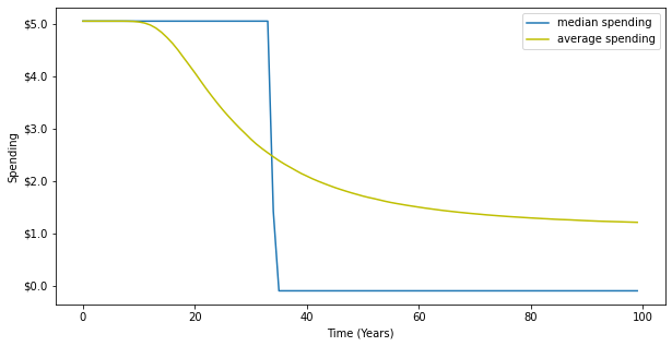
Chart 1: Spending $5.10 a Year (starting endowment value = $100)

Policy 2: Spend a Fixed Annual Percentage of the Endowment Value Equal to the Expected Simple Return of the Portfolio

The second policy we’ll consider is to spend the expected real simple return of the portfolio each year. From Table 1 that means spending 5.1% per year, and in fact this is close to Yale’s actual spending target policy of 5.25% over the past decade.⁷

Chart 2 uses a heatmap to show the probability of falling below a given level of spending, with the lightest color signifying 100% probability. Under this policy, it may come as an unpleasant surprise that median real spending falls by about 40% over 50 years, and by 2/3rds over 100 years. The median endowment value also falls by these amounts, since the spending rule is a fixed percentage of endowment value. We suspect most endowments would find this profile unattractive. The cause of this problem is often referred to as “volatility drag”, and relates to how volatility in returns makes the median return always lower than the average return.⁸ Following a spending policy equal to the expected portfolio return will keep the average spending amount and the average portfolio value constant, but this average is heavily influenced by a very small probability of extremely good outcomes. The median outcome, which is the most likely outcome, will always be lower, and if the average outcome is constant over time the median must be falling, as we see here.

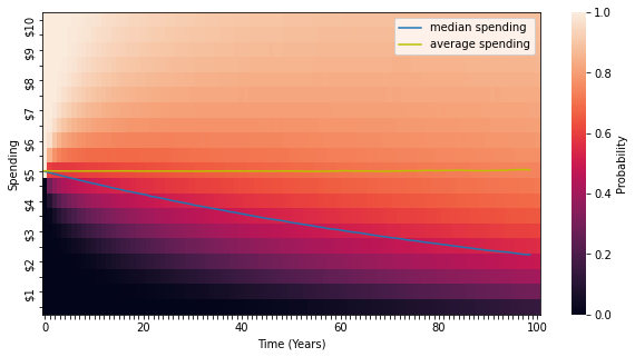
Chart 2: Spending 5.1% a year

Policy 3: Spend a Fixed Annual Percentage of the Endowment Value Equal to the Expected Compound Return of the Portfolio

This brings us to the third spending policy, which is to spend the expected compound real return of the portfolio. With the assumptions from Table 1 it is 4.2% per annum.⁹ This happens to match the average spending rate across all US college and university endowments.

We can see in the chart below that now median spending stays constant over time, while average spending drifts higher. Early thinking about endowment spending, such as that of Nobel laureate James Tobin (1974), viewed the previous rule, spending the expected simple return of the portfolio, as the ‘Sustainable Spending Rate’ that endowments should adopt.¹⁰ More recently, however, the consensus has shifted to viewing this third rule as a better definition of Sustainable Spending because it keeps median spending and median endowment value constant over time, and medians accord better with what we are “likely” to experience.¹¹

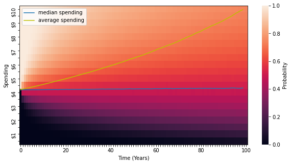
Chart 3: Spending 4.2% a year

How to Compare Different Spending Policies

For many endowment trustees, they may find the third policy more attractive than the first two…but is it the optimal choice? We can see from the charts that Rule 3 produces the highest total median and average dollar spending over the horizon – because spending less in early years allows more growth to fund higher spending later on – but does that make it the best policy? It would be a pretty tall order to identify the best spending policy just by eyeballing the differences between colorful heatmaps. Focusing on medians rather than averages seems reasonable, but it’s a value judgement to which we haven’t yet given a particularly rigorous foundation.

We need a more powerful summary statistic for comparing different spending rules. Such a metric should take account of:

• The level of spending – more is better than less.
• The smoothness of spending over time – consistent spending is better than volatile spending.
• The immediacy of spending – sooner is better than later.

The standard metric which economists use which neatly incorporates all of these criteria in evaluating an uncertain stream of spending over time is Discounted Expected Utility of Spending.

Utility

In order to use this metric, we need to uncover the endowment’s Utility function. This is not as difficult an undertaking as it may seem. First, it has been observed that the amount of risk endowments take does not seem to vary much over a wide range of endowment sizes, which allows us to reasonably use a form of utility called Constant Relative Risk-Aversion (CRRA) Utility. This type of Utility function has only one parameter, which is the degree of risk-aversion.¹² For a particular endowment, its risk-aversion can be deduced from the investment policy it has chosen, if we know the estimates of expected return and risk on which it based its portfolio choice.¹³ Given the investment environment described in Table 1, the endowment’s level of risk-aversion implied by its chosen portfolio is a fairly normal level exhibited by wealthy, financially sophisticated individuals.¹⁴

Time Preference: Weighing a Better Present Against a Better Future

With the endowment’s utility function and the distribution of portfolio returns in hand, we can calculate the Expected Utility of Spending for any spending policy – but to calculate the Discounted Expected Utility, we need to know how the endowment discounts current versus future benefits of spending, that is, the endowment’s “Time Preference.” Economists and philosophers have long noted the general human preference for good things to happen to us sooner rather than later, but does that apply to an endowment too? James Tobin thought that endowments should have zero time preference, stating: ¹⁵

“The trustees of an endowed institution are the guardians of the future against the claims of the present. Their task is to preserve equity among generations…In formal terms, the trustees are supposed to have a zero subjective rate of time preference.”

With respect to Professor Tobin’s view, we wonder if it is plausible or advisable for any social entity – endowment, foundation, family or individual – to exhibit zero time preference. Is it reasonable that an endowment would put an equal value on the social welfare arising from $1 today as it would on the same amount of welfare generated in 1,000 years? Indeed, there are good reasons why it would be rational for endowments to express some degree of time preference, such as a belief that making the world better today will pay dividends in making the world even better in the future, and acknowledging the truth that while endowments expect to exist for a very long time, that’s not the same as forever.¹⁶

How can we help an endowment calibrate its time preference? One suggestion is for the endowment trustees to contemplate how much they would spend if their only investment option were a risk-free asset paying a 0% real return each year. Any spending in this case would run down the endowment value, and the choice of how fast determines the endowment’s time preference.

The U.S. federal government suggests cost-benefit analysis of social programs use a real “social rate of time preference” of 3%.¹⁷ Another data point that garnered much attention was the U.K.’s Stern report on the economics of climate change (2006) which more controversially used a rate of time preference of 0.1% for weighing costs and benefits occurring over many years. We will use a rate of time preference of 2% for the Base Case analysis that follows.¹⁸

Put Your Faith in DEUS: Discounted Expected Utility of Spending

An endowment should prefer one spending policy over another if it generates higher Discounted Expected Utility of Spending (DEUS). In the table below, we compare the three spending rules we’ve already discussed against each other using this metric. What we show for each rule is how many dollars the endowment would need to start with so that it would generate the same amount of DEUS under each spending rule over a one hundred year horizon. We’ve assumed a time preference of 2% per annum, and risk-aversion consistent with risk and return numbers in Table 1. Notice that the endowment would need considerably more assets to start with under rules 1 and 2 to generate the same expected welfare as under rule 3.¹⁹ The endowment’s choice of spending policy matters a lot.

Comparing Spending Rules: Size of Endowment Needed to Generate Equal Welfare Over 100 Years Under Different Spending Policies
Rule 1 Spend $5.10 pa	Rule 2 Spend 5.1% of Endowment pa	Rule 3 Spend 4.2% of Endowment pa
$184	$151	$100

In Search of the Optimal Spending Policy

If we can compare the DEUS for different spending policies we propose, it begs the question: can we find an optimal spending rule? Remarkably, the answer is yes.²⁰ Robert Merton found it, and shared it in his first published economics article in 1969, marking the start of one of the most prolific and creative careers in financial economics.²¹ In fact, Merton did more than solve for the optimal spending rule: he solved for the joint optimal spending rule and optimal investment policy.

Three variables feed into the optimal amount of risk to take, known as the “Merton Share”:

1. The expected return of the risky portfolio in excess of the risk-free rate. Higher excess returns imply a higher optimal risk setting.
2. The variability of the risky portfolio measured by its variance.²² Higher variance implies lower optimal risk-taking, all else being equal.
3. The risk aversion coefficient – higher risk aversion implies lower optimal risk.

For the optimal spending rule, Merton shows that it must be a proportional rule, spending a fixed fraction of the portfolio each period. This optimal spending fraction is also a function of three inputs:

1. The “risk-adjusted” return, also known as the Certainty-Equivalent return of the total portfolio when invested at the optimal risk level. This is the certain return one would accept in lieu of the risky portfolio’s return. Higher risk-adjusted returns allow for higher spending rates, but generally not on a one-for-one basis.
2. The time preference rate. Higher time preference increases the optimal spending rate.
3. The level of risk aversion. If time preference is lower than the portfolio’s risk-adjusted return (as in our Base Case), then higher risk aversion increases the optimal spending rate, and vice versa.

Merton Optimal Investment and Spending Formulas for an Endowment with Infinite Life

k^* = μ – r γσ²

where k^* is optimal exposure to the risky asset
μ is the expected return on the risky asset
r is the return on the safe asset
σ is the annual standard deviation of returns of the risky asset
γ is the coefficient of CRRA risk aversion

C^* = r_ce – r_ce – r_tp γ

where C^* is the optimal spending rate²³
r_ce is the certainty equivalent return of the optimal portfolio
r_ce = r + k^* 2 (μ – r) r_tp is the investor’s time preference of spending

Where Merton Meets the Road

Knowing the optimal rule to follow is great, but does it deliver much real improvement over Rule 3, the “Sustainable Spending” policy? Staying with the same set of assumptions, Merton’s optimal spending policy would be to spend 2.4% of the value of the endowment each year. An endowment following the Sustainable Spending policy for 100 years, spending 4.2% per year, would need about 33% more in starting assets in order to deliver the same discounted expected utility from following the Merton-optimal rule, and the gap gets bigger as we look at longer horizons. The simplicity of the Sustainable Spending Rule is attractive, but it does not directly take account of the endowment’s risk aversion or time preference, and so in general it will lead to suboptimal spending decisions.

The chart below shows the average and median spending under the two spending policies (Sustainable and Optimal). It is difficult to visually decide which spending policy is more attractive without having a comprehensive metric that takes account of the main contours of the endowment’s preferences over uncertainty and time.

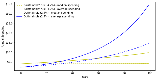
Chart 4: Comparing Merton Optimal vs. Sustainable Spending Rules

There are some preference sets for which the Sustainable Spending rule is quite close to Merton’s optimal spending rule, and others for which it’s even further away than the base case we examine. In our example from Table 1, if the endowment exhibited time preference equal to 7% per year, then Merton’s optimal spending policy would be to spend 4.2% per year, the same as the Sustainable Spending policy. On the other hand, if the endowment had zero time preference the Merton-optimal spending rate would be much lower, at just 1.6%.

Conclusion

The Merton model and its extended family of descendants do not appear to play a central role in shaping the investment and spending policies of major endowments, foundations or other long-lived pools of capital. For example, in David Swensen’s already-mentioned endowment bible, there is no mention of Merton or the cohort of researchers, notably John Campbell, who have extended his work. Swensen’s only mention of Merton is to dismiss his formulation of the problem:

“Economists might suggest that a utility function be employed to identify the appropriate asset allocation. Since few market participants would have any idea how to specify such a function, this technique proves remarkably unhelpful.”

We found several other influential books on endowment and foundation investing equally silent on Merton’s formulation and solution of the problem.²⁴

We don’t agree with Swensen’s criticism that the expected utility framework is too abstract to be useful in guiding, and linking, an endowment’s investment and spending policies. For example, in a survey we conducted two years ago and reported in Measuring the Fabric of Felicity, we found that a sample of financial professionals were comfortable calibrating personal utility functions. In addition, we found that their preferences were consistent with Constant Relative Risk Aversion, the form of utility function underlying the Merton formulation described in this note. Since Merton’s 1969 paper, researchers have extended the model to make it more realistic in many dimensions, and we discuss a partial list of these extensions in the Appendix.

Unlike endowments, individuals are afflicted with tedious burdens like taxes, finite and variable longevity and an uncertain posterity. These factors make finding optimal rules somewhat more complex, and change the details in various ways, but the core principles stay the same:

• risk aversion and time-preference matter
• risk-taking should be proportional to excess expected returns and inversely proportional to variance
• spending should follow a proportional rule and be linked to risk-adjusted return
• investment risk and spending risk are inseparable

We intend to discuss the more complex case of the individual investor in a follow-up note.

Much has changed in the 30-plus years since Swensen arrived at the Yale endowment, and in the 50 years since Merton’s original solution to the endowment investing and spending policy problem. Markets can go through a number of radically different investing environments over the life of any single individual, and even moreso in the case an endowment. For stewards of long-term capital, we think the Merton framework and its extensions provide valuable guidance on navigating these changing waters.

---

Appendix: Extensions

While Merton’s 1969 analysis gave us two simple formulas for the optimal spending and investing policy, it was under a stylized and restrictive set of assumptions. However, his formulation of the problem with the objective of maximizing Discounted Expected Utility of Spending is versatile and leads to solutions under a wide array of more realistic assumptions, many of which he provided in subsequent papers.

• The original Merton 1969 formulation was for a two-asset case, but later versions explicitly handle multiple assets. The two-asset case can be used where the risky asset can be considered the optimal portfolio of risky assets. The model handles any choice of risk-free asset, from Treasury Bills to inflation-indexed bonds.
• Although the original 1969 model assumed a constant risk-free rate and a risky asset that followed a random walk with constant expected return and variability, these assumptions can be relaxed. If the risk-free rate and expected excess return of the risky asset themselves follow independent random walks, the results remain substantially the same.
• In another important extension, Merton coined the term ‘hedging demand’ to describe the result that investors should want to own extra amounts of the risky asset if its expected return tends to go up when the price of the asset goes down, and vice versa.
• While we have focused on preferences characterized by Constant Relative Risk Aversion, solutions can be found for any concave and smooth utility functions, including ones that separate relative risk aversion from the elasticity of intertemporal substitution of consumption.²⁵
• Parameter uncertainty leads investors to take less risk than would be optimal based on the point estimate of investment attractiveness. Similarly, learning also leads to conservatism, having the opposite effect as mean-reversion, and generates negative hedging demand.
• Spending policies, such as ‘sustainable spending’ or smoothed spending, can be exogenously specified and then an optimal investment policy given that spending policy can be solved for. John Y. Campbell and Roman Sigalov of Harvard have solved such a model, which suggests that as expected investment returns fall, the optimal endowment investment policy is to take more risk, a phenomenon known as ‘reaching for yield.’

Family Wealth

Taxes on income, capital gains and inheritance result in significantly lower expected returns for private taxable wealth than that experienced by non-taxable endowments or foundations. As a result, optimal spending policies for large pools of private capital will be substantially lower than optimal spending policies for tax-exempt entities, assuming similar degrees of risk-aversion and time preference that we used for our typical endowment. With the investment environment assumptions from Table 1, but with a flat 30% tax on returns, 0% inheritance tax and assuming inflation of 2%, the Merton optimal spending policy for an endowment-like taxable pool of capital would be lower than that for a non-taxable endowment at about 1.5% per annum.

For families who ascribe similar utility to the consumption of future generations, the optimal spending rate would be lower than that of an endowment to take account of the expected growth in the size of the pool of future beneficiaries. For individuals whose savings will be primarily used during their retirement, the Merton optimal spending rule for the infinite horizon can be used to annuitize wealth to a finite horizon. We will discuss this in more detail in an upcoming note that focuses on individuals.

Other Popular Spending Policies

Probably the first long-term spending policy that occurs to most investors is to spend the interest and dividend income they receive on their portfolio, which they hope will leave the earning power of their portfolio constant over time. Currently, for a portfolio 85% invested in global equities and 15% in US inflation-linked bonds, the resulting policy would be to spend 1.4% per year. While the simplicity of this rule is admirable, it is unlikely to be optimal except by coincidence as it does not explicitly take account of the risk or time preference of the investor, and its connection with the expected return of the portfolio is weak due to changes in company dividend policy over time. And of course, a dividend-based rule is not much help for investors who allocate heavily to alternative investments which have distribution policies that are arbitrary and rarely adjusted for inflation. A variant of this rule uses the Cyclically Adjusted Earnings Yield in place of the dividend yield of equities. The problem with this policy is that earnings yield is an estimate of the expected real return of the equity market, and as we’ve seen already, spending the expected return of the portfolio (see spending Rule 2 in the body of the note) is unlikely to be optimal.²⁶

Many endowments apply a percentage spending rule on a smoothed basis. For example, the Yale endowment states:

Spending in a given year sums to 80% of the previous year’s spending and 20% of the targeted long-term spending rate applied to the market value at the start of the prior year. The spending amount determined by the formula is adjusted for inflation and an allowance for taxes, subject to the constraint that the calculated rate is at least 4.0% and not more than 6.5% of the Endowment’s inflation-adjusted market value at the start of the prior year.

Smoothed spending policies pick up the problem of fixed dollar policies, which can result in the endowment running out of money surprisingly quickly.

Endowment Growth Through Ongoing Contributions

Endowments usually expect to receive further donations over time, and this can be integrated into the model for the optimal investment and spending policy. For example, Yale’s endowment has received annual donations of 2% to 2.5% of the value of the endowment over the past decade. However, many donors want their contributions to have long-term impact, and don’t expect them to form part of the annual operating budget. These, and related considerations such as the risk characteristics of the flow of donations over time, have been addressed and modeled by Robert Merton (1991) and others. Foundations and wealthy families can usually think about spending policies without this complication.

For Investors Expecting Higher Returns Than Implied by Their Risk Taking

Some investors may expect much higher returns than are reflected in their portfolio choice, possibly as a response to an aversion to leverage. For example, if an endowment expected a 10% return on a well-chosen portfolio of risky assets with 15% risk, the optimal allocation to those risky investments would be 160% with the level of risk aversion we’ve been using. But let’s say the endowment decides to allocate just 85% to this attractive mix of investments. What is the optimal spending policy the endowment should pursue in this case? We can still use the Merton spending rule as expressed, but we need to define the risk-adjusted return on the portfolio more generally as:

r_ce = r + k(μ – r) – γ k² σ² / 2

where k is the actual allocation to the risky part of the portfolio, and not necessarily the optimal Merton Share allocation

Using this higher risk-adjusted return based on expected risky asset returns of 10% as an input to the Merton rule for optimal spending, but assuming an allocation of just 85% to the risky assets, produces a spending policy of 4.7% as compared to an optimal spending policy of 2.4% if the expected return on risky assets were 6%. Remarkably, the optimal spending percent would only increase from 4.7% to 5.9% if the endowment allocated 160% of its capital to the risky assets, making use of leverage. The relatively small uplift to spending rate doesn’t seem worth the 75% increase in exposure to risky assets, making it understandable why an endowment might choose less than the optimal amount of risk. As is usually the case with decisions based on optimizations, the marginal benefits decline as the optimal point is approached, so investors should focus on getting in the general vicinity of optimality and not be too fixated on getting to the exact optimal point.

---

Further Reading and References

• Acharya, Shanta and Elroy Dimson. Endowment Asset Management: Investment Strategies in Oxford and Cambridge. Oxford University Press. 2007.
• Annable, Vince. The Household Endowment Model : Wealth Planning for Affluent Families. Wealth Strategies Advisory Group. 2019.
• Baumeister, Roy, George Loewenstein and Daniel Read. Time and Decision: Economic and Psychological Perspectives of Intertemporal Choice.” Russell Sage Foundation. 2003.
• Benzel, Rick and James E. Demmert. The Sustainable Endowment. New Insights Press. 2019.
• Black, Fischer. “The Investment Policy Spectrum: Individuals, Endowment Funds and Pension Funds.” Financial Analysts Journal. 1976.
• Campbell, John, Y. and Luis M. Viceira. Strategic Asset Allocation. Oxford University Press, (2002).
• Campbell, John, Y. and Roman Sigalov. “Portfolio Choice with Sustainable Spending: A Model of Reaching for Yield.” NBER. 2020.
• Campbell, John, Y. “Investing and Spending: The Twin Challenges of University Endowment Management.” Forum Futures. 2012.
• Dybvig, Philip H. “Dusenberry’s Ratcheting of Consumption: Optimal Dynamic Consumption and Investment Given Intolerance for Any Decline in Standard of Living.” Review of Economic Studies. 1995.
• Dybvig, Philip H. and Zhenjiang Qin. “How to Squander Your Endowment: Pitfalls and Remedies.” Washington University in St. Louis and University of Macao. Unpublished paper, 2019.
• Ennis, Richard and J. Peter Williamson. “Spending Policy for Educational Endowments.” The Common Fund Publications. 1976.
• Ford Foundation Advisory Committee on Endowment Management. “Managing Educational Endowments: Report to the Ford Foundation.” Ford Foundation. 1969.
• Goetzmann and Swensen. Yale Endowment Management Course description.
• Grinold, Richard, David Hopkins, and William Massy. “A Model for Long-Range University Budget Planning Under Uncertainty.” Bell Journal of Economics. 1978.
• Hindy, Ayman and Chi-fu Huang. “On Intertemporal Preferences With a Continuous Time Dimension II: The Case of Uncertainty.” MIT. 1989.
• Kochard, Lawrence E. and Cathleen M. Rittereiser. Foundation and Endowment Investing: Philosophies and Strategies of Top Investors and Institutions. Wiley. 2008.
• Merton, Robert, C. “Lifetime Portfolio Selection under Uncertainty: The Continuous-Time Case.” The Review of Economics and Statistics. Aug 1969.
•      , “Optimum consumption and portfolio rules in a continuous-time model.” Journal of Economic Theory. 1971.
•      , Continuous-Time Finance. Oxford. 1990.
•      , “Optimal Investment Strategies for University Endowment Funds.” NBER. 1991.
• Orr, Leanna. “David Swensen Is Great for Yale. Is He Horrible for Investing? How the Yale Model ate endowments — and everything else.” Institutional Investor. July 2019.
• Swensen, David, F. Pioneering Portfolio Management: An Unconventional Approach to Institutional Investment. Free Press. 2000.
• Tobin, James. “What is Permanent Endowment Income?” American Economic Review. Vol. 2, No. 64, 427-432. 1974.
• Yale Investment Office. Spending Policy, 2019 Update. p24. 2019.

---

1. This not is not an offer or solicitation to invest, nor should this be construed in any way as tax advice. Past returns are not indicative of future performance.
   We are very grateful for the help of Jamil Baz, Larry Hilibrand, Ayman Hindy, Chi-fu Huang, Antti Ilmanen, Andy Morton, Vlad Ragulin, Jeffrey Rosenbluth, Eric Rosenfeld and Scott Wilson. All errors are our own.
   
2. Campbell (2012).
   
3. 2019 NACUBO-TIAA Study of Endowments, 2010-2019 spending. Here. US College and University Endowments and related foundations. Yale spends about 5.25%.
   
4. This expected return is expressed as an arithmetic pa expected return. We assume the returns of the portfolio of risky assets follow a random walk.
   
5. 5.1% = 85% x 6% + 15% x 0%
   
6. The median value of spending is the outcome that defines the middle of the distribution, and is often useful to think about separate from the average outcome because the median is less heavily influenced by extreme outliers. For a time series of returns with volatility, the median return will always be lower than the average return.
   
7. As we’ll discuss later, Yale’s spending policy makes use of smoothing and also collars of 6.5% and 4%, which in effect makes its spending rule something of a hybrid between a percentage rule and fixed dollar rule.
   
8. An example illustrates this effect. Let’s say that each year, there’s a 50/50 chance that the endowment’s portfolio either increases in value by 18% or decreases in value by 8%. The average of +18% and -8% is the 5% average return of the endowment’s portfolio, with a bit of rounding. But, if the endowment goes up by 18% the first year, and then declines by 8% the second, or the other way around, the value of the portfolio will have returned only 4.2% per annum, 0.8% lower than the 5% expected annual return. This 4.2% return is the compound (or median or geometric average) return of the portfolio, while 5% is the expected arithmetic return of the portfolio.
   
9. Also known as the geometric average return.
   
10. “…The trustees of an endowed university like my own (Yale) assume the institution to be immortal. They want to know, therefore, the rate of consumption from endowment which can be sustained indefinitely. Sustainable consumption is their conception of permanent endowment income…Consuming endowment income so defined means in principle that the existing endowment can continue to support the same set of activities that it is now supporting.”
    
11. Dybvig and Qin, “How to Squander Your Endowment,” 2019, and Campbell and Sigalov, “Portfolio Choice with Sustainable Spending: A Model of Reaching for Yield,” 2020.
    
12. CRRA Utility takes the form: U(C) = (1 – C^{(1 – γ)}) / (γ – 1) , where C is spending and γ is the coefficient of risk aversion.
    
13. Alternatively, for an endowment wishing to decide on an investment policy, there is a very reasonable range of CRRA risk-aversion levels which can serve as a useful starting point without requiring a complicated, idiosyncratic calibration exercise.
    
14. Equal to 2.75 times the risk-aversion of a typical Las Vegas professional, card-counting gambler trying to maximize the growth rate of his bankroll. It’s a level of risk-aversion that would make an investor ambivalent about accepting a gamble with a 50% chance of making 25% versus a 50% chance of losing 15%. See our note, The Fabric of Felicity.
    
15. In the 1974 article already cited, and referenced by David Swensen in describing the Yale endowment’s spending policy choice.
    
16. If the endowment truly had zero time-preference, then in a world in which the only investment available to an endowment were a risk-free asset that paid a 0% real return above inflation, it would be optimal for the endowment to spend zero, thereby preserving the real value of the endowment forever. Another reductio ad absurdum argument observes that an endowment that had no time preference and expected to live forever would be willing to pay an infinite price for a perpetual, risk-free bond that offered a positive real yield. While we present this scenario as a thought-experiment, it is not as far-fetched as it used to be.
    
17. See OMB Circular A-4 and OMB Circular A-94.
    
18. Time preference is equal to the desired spending rate in the zero return scenario multiplied by the coefficient of risk-aversion of the endowment, which we’ve assumed is equal to 2.75 in the Base Case. So, if the trustees felt that they would spend 0.75% of the endowment each year in a zero return environment, time preference would equal 2% pa.
    
19. These results are sensitive to choice of time preference, but robust within a reasonable range of choices. For example, with time preference of 0% , rules 1 and 2 would need to start with capital of $184 and $168, and with time preference of 4%, rules 1 and 2 would need to start with $183 and $131 to generate the same discounted expected utility of spending over 100 years as rule 3.
    
20. Given a set of assumptions that asset prices are well-behaved and investors exhibit Constant Relative Risk Aversion.
    
21. Of course, others also deserve credit for contributing to these insights, including Paul Samuelson, Merton’s mentor and collaborator, and Franco Modigliani, who was awarded a Nobel prize for his pioneering contributions to the field of life-cycle financial decision-making.
    
22. 22 Variance is equal to Standard Deviation squared.
    
23. Merton’s formula for optimal consumption can be arrived at by observing that a consumption policy is optimal only if all along its path the marginal utility of $1 not consumed at a point in time is equal to the marginal benefit of that $1 plus its growth at a later time, adjusted for time preference. This can be expressed as: U'(C_t) = U'(C_t + dt) * e^{(r_ce – r_tp)dt} . This simplifies to: ln((C_t + dt) / C_t) = (r_ce – r_tp) / γ . As ln((C_t + dt) / C_t) is the growth in optimal consumption, and r_ce is the growth in the portfolio, then optimal consumption, C^* = r_ce – (r_ce – r_tp) / γ . This is Merton’s formula for consumption, C^* .
    
24. Such as “Foundation and Endowment Investing: Philosophies and Strategies of Top Investors and Institutions”, “Endowment Asset Management: Investment Strategies in Oxford and Cambridge”, “The Sustainable Endowment” or “The Household Endowment Model: Wealth Planning for Affluent Families.”
    
25. Known as Epstein-Zin utility.
    
26. It is an open question whether CAEY is a predictor of the expected arithmetic or geometric return of the equity market, but in either case, this criticism holds.