July 16, 2019
Featured Insights
Smart Beta: The Good, the Bad, and the Muddy
By James White and Victor Haghani 1
Abstract
Factor investing, or Smart Beta as it’s known in long-only form, has become one of the most popular forms of investing, straddling the active-passive divide. The authors evaluate theoretical and empirically-based arguments for factor investing, concluding that while many of the arguments, particularly the theoretical ones, are sound, there are still reasons for considerable skepticism. They describe the trajectory of the factor investing paradigm, from the cradle of the efficient markets school to its championing by some of the world’s most successful investment management firms. While factor investing is typically discussed using the language and machinery of efficient-markets models, investors are primarily expecting anomalous excess returns more consistent with behavioral explanations and other market inefficiencies. For factors with plausible risk-based explanations, the authors conclude that even in the presence of significant factor premia, the market portfolio is still likely to be optimal for most investors. The authors also provide simple logical arguments to assess claims such as that factor investing delivers gross investment returns similar to traditional active managers, but with lower fees.
Factor investing is one of the hottest areas in modern finance. It has spawned hundreds of academic articles within the ivory tower and trillions of dollars in AUM without, much of it invested through long-only ‘Smart Beta’ strategies. At its core is a high-stakes unresolved tension spanning the industry and academia: is the stock market essentially efficient, or are there major inefficiencies from which large groups of investors can systematically profit?
The story begins with Nobel Laureate Eugene Fama and his 1965 PhD thesis, in which he proposed that the stock market is efficient and therefore very hard to beat. Decades later, following the work of others,2 Fama and his colleague Kenneth French noticed that stocks of companies that were either relatively small or cheaply valued had higher returns than predicted by the most popular stock market model of the day: the Capital Asset Pricing Model (CAPM). This didn’t dissuade Fama from his belief that markets were efficient; rather, he and French concluded that the CAPM wasn’t the right model. They proposed that there were two more risk factors that were needed in addition to market Beta, which they termed the Size and Value factors. But two of Fama’s PhD students, David Booth and Cliff Asness, took the same data and reached the opposite conclusion: that factor returns represented a market inefficiency and thus also an investment opportunity. Each went on to become a billionaire building businesses premised on their view that investors would flock to a new factor-focused style of investing.3
As shown in Exhibit 1, investors have favored Booth and Assness’ view, voting with trillions of their assets – but many experts, including the Nobel Prize Committee, think that Fama and the Efficient-Market Hypothesis have considerable merit too. How can everyone be right? In this article, the authors discuss the major streams of thought behind factor investing and this central tension between the efficient and inefficient markets camps. We try to fairly present the case for factor investing, and also some reasons for skepticism, with the hope that readers will be left well-equipped to decide whether and how to incorporate factor investing into their own portfolios.
Exhibit 1: US Smart Beta ETF Asset Growth
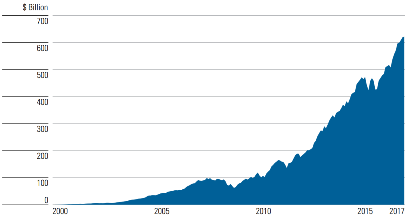
Source: From Morningstar Research Data as of the 6/30/2017 report. Only listed ETFs included. Excludes factor exposure held in mutual funds, managed accounts, private funds, and non-US listed funds and ETFs. Three of the largest factor-focused investment managers – DFA, AQR and RA – are not represented in this data as they make little use of ETFs. On the other hand, this dataset overstates ETF Smart Beta exposure in that it includes both Value and Growth ETFs, instead of the net of the two.
Background
The central idea behind factor investing is that the best way to explain individual expected stock returns is with multiple systematic drivers, called factors. A multi-factor framework was put forward in an elegant bit of reasoning called the Arbitrage Pricing Theory (APT)4 and caught on quickly because the single-factor CAPM5 wasn’t doing a very good job explaining the return structure of individual equities.6 Then in a seminal 1992 paper, Fama and French proposed the three-factor model which became the foundational tool in the multi-factor framework. They argued that the CAPM, based on a single “total market” factor, can be significantly improved upon by adding two additional factors:
- Value: The differential return between low Price/Book stocks and high Price/Book stocks
- Size: The differential return between small market-cap stocks and large market-cap stocks
They found that exposure to both the Value and Size factors had historically earned a positive return premium, and that their three-factor model did a much better job than the single-factor CAPM of explaining individual stock returns. Over time, the number of factors that attract investor attention has grown dramatically. These are the most popular ones, as suggested by the number and size of funds set up to focus on them:
- Value: stocks with low Price/Book ratios perform better
- Size: small company stocks perform better
- Dividend yield: stocks with high dividend yield, or high dividend growth, perform better
- Quality: stocks with high profitability and/or conservative investment perform better
- Momentum: stocks that have outperformed the market over the past year perform better
- Low Volatility: stocks with low historical volatility and/or low Beta perform better
The ‘style’ factors above are cross-sectional factors comparing one group of stocks to another (e.g. small-cap stocks vs. large-cap stocks). While most of the research literature on factor investing focuses on long-short portfolios, in this article we will concentrate on the most common and accessible form of Smart Beta: long-only equity portfolios tilted away from the market portfolio.7
Why Invest in factors?
We believe the prime reason investors seek factor exposure is to earn higher risk-adjusted returns than the market-cap-weighted index. This isn’t unreasonable, since over significant historical periods that’s exactly what’s happened. For example, using data from the Kenneth French website8 from June 1963 to March 2019, we built a long-only US equity portfolio with equal exposures to the six popular factors listed above. Ignoring implementation costs, this hypothetical multi-factor portfolio beat the market portfolio by 2.8% annually with almost equal experienced volatility.9 You can see where all the excitement about factor investing comes from. Proponents of factor investing argue that not only has the historical record looked great for these factors, but also that there are sound underlying reasons explaining why this should be the case and should continue into the future. These explanations fall into two broad categories: risk-based and behavioral.
Risk-based explanations suggest that exposure to factors involves bearing systematic risk which cannot be fully diversified away, so investors earn a structural positive risk-premium to compensate for bearing that extra risk. Value and Size and the rest are called ‘factors’ precisely because they were originally conceived as being ‘risk factors’ explaining expected stock returns in an efficient market. Indeed, the vocabulary of factor investing, with labels like ‘factor premia,’ ‘style premia’ and ‘Smart Beta,’ is an artifact of its origins in the academic efficient-markets camp.
So what does a risk-based story look like? Taking the Size and Value factors for example, one plausible conjecture is that a very deep economic crisis will wash away the smallest companies and the companies with lowest relative valuations. As the risk of catastrophic economic depression is a background risk that doesn’t show itself in routine equity price movements, it is not picked up in the conventional measurement of market Beta, and therefore isn’t compensated through the Beta risk premium.10 Instead, the risk is compensated through the Size and Value factor premia. Another reasonable risk-based argument suggests the publicly-listed stock market meaningfully under-represents small private businesses, and that the Size and Value factors are needed to build a portfolio which is a more true representation of the total market portfolio.
Many of the factors however – in particular Low Vol, Momentum and Dividend Yield – are difficult to explain with a plausible risk-based story. These factors rely more on behavioral and constraint-based explanations which posit that factor returns represent market inefficiencies. In this view, factor investing is a systematic way to profit from deep-seated cognitive investing mistakes of others or from constraints and frictions that give rise to inefficiencies. For example, the Low Vol factor is difficult to explain with an obvious risk-based argument, as it’s not clear from either data or experience what ‘extra’ risks uniquely plague lower-volatility stocks.11 However there are a number of plausible behavioral explanations, such as that investors have an aversion to outright financial leverage, driving them to over-price high-volatility equities relative to low-volatility equities which would require some leverage to deliver the same absolute return (Black et al., 1972).12 Momentum also lacks a persuasive risk-based explanation, but there is a solid behavioral case to be made that it derives from aggregate investor return-chasing, and that this is a structural feature of investor psychology visible in the behavior of nearly every tradable asset.13 For any given factor, multiple explanations may also be at play simultaneously.
Reasons for Skepticism
So far, we’ve discussed the factor framework from the perspective of its advocates. We’ll now turn to several causes for concern.
Let’s start with risk-based justifications for factor investing, which hold that factor premia are primarily risk-based and efficiently priced. In this case, an investor would want a portfolio with exposure to a given style factor only if she specifically believes she’s more or less sensitive to that factor than the average investor. A fundamental fact of market arithmetic is that the sum of all individual portfolios must equal the market portfolio. So, for every investor who is less sensitive to the risk of a given factor and wants to earn the factor premium, there must be an investor who is more sensitive to that factor and wants to avoid its risk by paying the factor premium. For example, it may be that investors holding above average small cap exposure may be offsetting small-business owners who prefer to avoid Small-cap stocks. While this is theoretically possible, in practice for most factors it seems a stretch to think the market functions this way. For one thing, the risk scenarios involved in many of the factors aren’t sufficiently clear or well-known for investors to have a strong view about them. And also, if factors really do arise from this sort of risk explanation, where are the funds pitched to investors who want to avoid some factor and earn a return below that of the broad market? For example, we strongly suspect that investors in both Value and Growth funds expect to earn above-market returns, not that growth-fund investors perceive themselves as earning below-market returns in exchange for avoiding the risk of the Value factor. If indeed investors don’t have highly individual factor-risk preferences, and if we accept the risk-based argument, then even though there may be large factor premia, the market portfolio will still be the optimal portfolio for most investors.14
While risk-based explanations are consistent with efficient markets, behavioral explanations are explicitly connected to market inefficiencies. The obvious question is: to what extent should we expect these market anomalies to continue? We know there are many reasons anomalies tend to dissipate over time. Large pools of opportunistic capital tend to move the market towards greater efficiency, and the composition of market participants changes relative to the historical period during which past returns were observed. And professional investors are becoming more thoroughly trained in valuation techniques than their predecessors, while many non-professional investors are retreating from stock-picking in favor of market-cap-weighted index funds. Some anomalies may indeed survive for long periods of time, but with multiple potential explanations for any given factor it’s difficult to know what persistence to specifically look for, or how to assess the magnitude of expected outperformance going forward.
The question of anomaly persistence has been addressed in a number of research papers, and most, though not all, have found that as a market inefficiency becomes known through published research it provides smaller excess returns over time.15 One vivid example of this post-publication return decay is the case of the ‘January Size Effect.’ The January Size Effect was the tendency of small cap equities to strongly outperform the rest of the market each January, which had several plausible behavioral explanations. However, within a few years after the 1983 publication of two academic papers by Keim and Reinganum describing this effect, it disappeared (McLean and Pontiff, 2016).
The correct explanation for some proposed factor premia may be neither risk-based nor behavioral. Not all statistical results are true in that they accurately reflect an underlying structural reality. The literature of factor results principally depends on statistical regressions, and typically factor ‘discoveries’ have been reported in journals when the result has met a conventional but narrow test of statistical significance. That’s a good start, but not as rock-solid as it might seem. If researchers run enough regressions, eventually the data will oblige with an interesting finding (Harvey et al., 2015). There are many ways that careful researchers can and do correct for this problem, such as by inspecting out-of-sample data from other time periods or other markets for the existence of the phenomenon. And indeed, data for several of the most popular factors stand up to these more rigorous standards; particularly Value, Momentum and Low Beta.
However, ‘mining’ for factors makes statistical limitations a very real concern with factor research more broadly. Financial data is a harsh taskmaster, and many of the available tools of statistical inference have limited power when applied to financial datasets. Since the publication of the Fama-French three-factor model, researchers have searched for and discovered a large number of other factors with positive historical return premia, decent levels of apparent statistical significance and improved explanatory power with respect to individual stock historical returns. This proliferation of factors, now in the hundreds as illustrated in the chart below, has given birth to the term ‘factor zoo’ in reference to the overall literature (Cochrane 2011). The same phenomenon magnified ten-fold is seen in the explosion in the number of ETFs and indexes on which they are based (Dickson et al 2012). Adding to the doubt and confusion over the factor zoo’s quickly expanding population is the well-publicized ‘Replication Crisis’ in social science research, referring to the realization that many academic papers in economics and other social sciences report findings which other researchers are unable to reproduce (e.g. Ioannidis et al 2017).
Exhibit 2: Journals Published Through December 2018. Data Collection in January 2019.
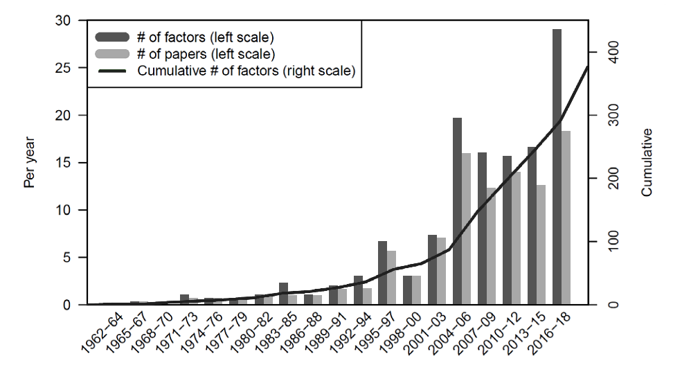
Source: Figure 1 in Harvey and Liu (2019).
While data mining concerns cast doubt on the authenticity of the factor zoo’s exotic members more than on the core factors, there’s another data issue which impacts all the factors. Nearly all financial data is subject to complex relationships, periodic regime changes, and there’s just relatively little total data. Adding multiple markets and multiple historical periods doesn’t add as much useful information as it could, because markets are often affected by common large-scale drivers which spill over across markets and time periods. Simply put, it’s very hard to use the data to clearly determine what’s causing what. It may be that the Value factor, for example, has a valid risk explanation but the feared scenarios have not yet shown up in real-world data. But it’s also possible that the Value factor’s returns across many markets have historically resulted from a common hidden driver affecting equities everywhere, such as long-term technological shifts or globalization. Investors would probably want more of the Value factor if the first explanation were the correct one, but there isn’t enough data to know. Researchers and investors are good at finding stories which seem to fit the data, but the data itself is much more close-mouthed about which story is right, and consequently what to expect in the future.
We turn now to concerns that go beyond whether history is a good guide to the future. We are skeptical of claims that Smart Beta offerings are designed to deliver what professional active managers provide, but at lower fees and with greater simplicity and transparency. Professional active managers have generally out-performed the market before fees, so doing the same but with lower fees sounds pretty good. However, we know that the sum of all portfolios must equal the market portfolio, a fact often called Sharpe’s Arithmetic. In contrast to market Beta, it is not possible for all investors to hold the same style factor exposures – someone must be on the other side of any tilt away from the market portfolio. But if professional active managers are outperforming the market before fees, while individual retail investors are increasingly moving toward index investing, who’s taking the other side of the professional active managers? Unless the Smart Beta investor can confidently identify another large group of investors who are offsetting the professional active managers’ portfolio tilts, there should be some cause for concern.
Even if we accept that both risk-based and behavior-based factors are expected to deliver excess returns in the future, we worry that the transactions costs and frictions involved in harvesting them render the net excess return too meager in most cases to warrant holding portfolios with large factor tilts. As can be seen in the table below, factor-focused portfolios require more active rebalancing than market-cap-weighted portfolios, leading to higher turnover, transaction costs, and tax inefficiency. Constructing these portfolios also requires considerable care and skill, leading to higher investment management fees, also evident in Exhibit 3. Several academic studies have tried to quantify the transactions costs incurred by the higher turnover. A detailed study by researchers at AQR (Frazzini et al 2012) using nearly \$1 trillion of actual transaction data estimated that the cost of trading was equal to about 40% of the gross historical extra factor return. Most of this cost comes from price impact. While the frictions found in this study already are high enough to warrant concern, we worry that future transactions costs may be considerably higher, as the popularity of factor investing is greater than it was on average over the historical period analyzed.
Exhibit 3: Turnover and Fees of Select Smart Beta Funds vs.VTI Market-Cap-Weighted Fund
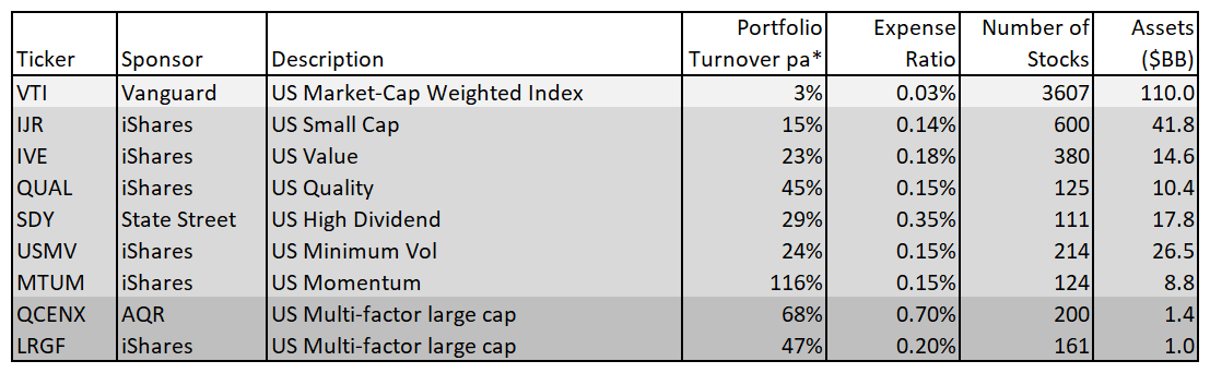
Source: Table created by authors based on data from iShares, SPDR, Vanguard and data from https://etfdb.com/themes/smart-beta-etfs/.
* latest 3 years average, as per Morningstar.com.
Nor is factor investing as simple or transparent as some of its proponents claim. There are numerous ways to structure a portfolio loaded on any one factor. The various style factors aren’t naturally independent of one another. So, should a portfolio focused on one given factor ignore its other possible factor exposures, or should it be designed to have zero exposure to all the other factors? In fact, for factor strategies that do not allow shorting, it is usually impossible to construct a portfolio with exposure to just one factor because many of them are correlated with each other. For example, there is a positive correlation among the Value, Quality, Dividend Yield and Low Beta factors, averaging 0.4 across the six possible pairings.16 Once it’s been decided which equities to hold in a Smart Beta portfolio, how should the weights be determined: market-cap weights, equal weights, factor loading or some other scheme? Exhibit 4 illustrates the complex nature of constructing factor portfolios in practice, by showing the wide range of individual holdings for four iShares US equity Value ETFs. Perhaps just the fact that iShares offer four different Value ETFs makes the point with no need for a chart.
Exhibit 4: Comparing Individual Equity Holdings of Four Popular iShares US Value ETFs
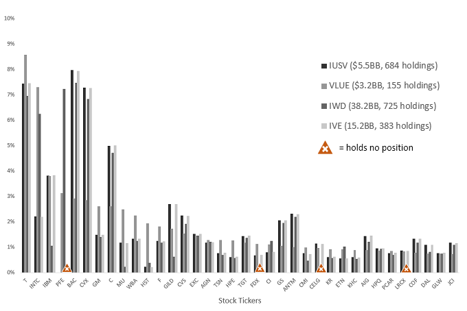
Source: Table created by authors based on data from iShares.com. Percentages normalized for same total % in these top 25 holdings of VLUE.
Another tack taken by supporters of Smart Beta is to argue that the market-cap-weighted index is flawed by design. They claim that Smart Beta portfolios constructed with just about any imaginable alternative weighting scheme will produce a portfolio with a higher return and/or lower risk than the market portfolio. Proposed designs include equal weights, random weights, or weighting based on accounting data, such as the size of company sales. Looking backward these alternative formats have indeed produced attractive returns, but that is because such portfolios generally wind up with significant loadings on the Size and Value factors (because Value stocks tend to be smaller too), and we know that exposure to these factors has historically paid off.17 A related proposition is that market-cap-weighted indexes are flawed because they force investors to be overweight overvalued equities and underweight under-valued equities. This is logically unsound, in that it presupposes that passive investors know a priori which equities are overvalued or under-valued, which is in direct contradiction with what it means to be a passive investor in the first place (Perold 2007) and (Haghani 2017).
So far, we have focused on expected returns. We also worry that the risks of factor investing will be more extreme than history suggests. We believe that the large flow of funds into factor investing strategies has primarily been driven by investors chasing attractive historical returns, and only secondarily by the theoretical models behind them. Many of the style factors have now suffered a long period of disappointing returns. For example, the equally-weighted six-factor portfolio which beat the market by 2.8% p.a. from 1963 to 2019 underperformed the market by 0.4% p.a over the past five years, before fees or costs, with about 5% more risk. Since the start of 2017, the under-performance has been about 6% cumulatively. If this poor relative performance continues, it could lead to a broad disenchantment with factor investing. Resultant outflows could cause losses in individual factors much larger than suggested by the historical record, as well as high correlation among the factors.
In fact, the historical record does include some pretty large losses from factor investing. For example, the Kenneth French data show that a portfolio long the 20% of stocks with the highest momentum and short the 20% with the lowest momentum has experienced two major crashes. The first was from June 1932 to June 1933 during which time the Momentum Portfolio lost 90% of its value, before transactions costs. More recently, from February 2009 to February 2010 it experienced a loss of 70%. A long-only portfolio of Value stocks underperformed the broad market by 34% from May 1998 to February 2000 during the Dot-Com Bubble, using the Kenneth French dataset. The ‘Quant Crash’ of August 2007 is another example of factor-related losses much larger than indicated by historical risk measures (Khandani, Lo 2008). The magnitude of the moves was famously captured in the remark by Goldman Sachs CFO David Viniar, who said “We were seeing things that were 25-standard deviation moves, several days in a row.”
Return-chasing behavior not only may lead to much higher risk in factor strategies than experienced in the past, but is also likely to cause some predictable patterns in factor returns themselves. It has been suggested that factor returns exhibit momentum to a horizon of about one year, while to longer-term horizons they exhibit weak mean reversion. This is a topic hotly debated by thought leaders in the field, with Cliff Asness of AQR on the side that factor returns are not predictable in the short run, and Rob Arnott of Research Affiliates arguing that they are. A number of recent academic papers (Gupta et al 2018, Arnott et al 2018, Ehsani et al 2019, Ilmanen et al 2019), seem to be resolving the matter in favor of the view that momentum, and to a lesser extent long-term mean reversion, have been mildly present in factor returns.
Where does this leave us?
If all the historical market data got lost somewhere, what kinds of investing could we still do? We could still make pretty reasonable decisions about bond investing based on yields and current fundamentals. We could invest in stock market indices and real-estate using forward-looking metrics like earnings and rental yield, and we could even make individual stock-picking choices based on current fundamentals. But factor investing, as currently practiced, would never have made it to the drawing board. We’re not suggesting to ignore historical data when available, or to avoid any strategy which requires some data; indeed historical data can often be useful. But there’s something comforting about making an investment relying primarily on forward-looking data, and only secondarily on a specific historical record.
Factor analysis is undoubtedly useful in decomposing and understanding past returns, and in understanding what kinds of risks and ‘bets’ are embedded in a given portfolio. With the proliferation of potential Factors to invest in, it is critical for investors to understand the fundamental reasons, if any, that a Factor has delivered attractive returns in the past and assess the likelihood that they will persist. This is a very daunting task when armed only with historical returns in markets where the players and the rules of the game have been constantly changing. Even for the subset of Factors with the most solid risk and behavioral underpinnings, we suspect their expected returns, net of the costs to harvesting them, are considerably lower than their past returns. We’re equally concerned that the risk involved in Smart Beta portfolios are likely to be substantially higher than historical data suggest.
As we’ve discussed, there are reasons you might want to deviate from the market, but the threshold for material deviations should be pretty high. The market-cap portfolio really is special: it’s the only single portfolio everyone can hold simultaneously, and tilting away from it in any way is a zero-sum bet against someone else. In the words of Professor John Cochrane: “No portfolio advice other than ‘hold the market’ can apply to everyone.” 18
Further Reading and References
- Basu, S. (1977). “Investment Performance of Common Stocks in Relation to Their Price-Earnings Ratios: A Test of the Efficient Market Hypothesis.” The Journal of Finance 32.3; 663-682.
- Banz, R. (1981). “The relationship between return and market value of common stocks.” Journal of Financial Economics 9.1; 3-18.
- Ross, S. (1976). “The Arbitrage Theory of Capital Asset Pricing.” Journal of Economic Theory 13.3; 341-360.
- Merton, R. (1973). “An Intertemporal Capital Asset Pricing Model.” Econometrica 41.5; 867-887.
- Treynor, J. (1961). “Market Value, Time, and Risk.” Unpublished manuscript; 95-209.
- Sharpe, W. (1964). “Capital Asset Prices: A Theory of Market Equilibrium Under Conditions of Risk.” The Journal of Finance 19.3; 425-442.
- Lintner, J. (1965). “The Valuation of Risk Assets and the Selection of Risky Investments in Stock Portfolios and Capital Budgets.” The Review of Economics and Statistics 47.1; 13-37.
- Mossin, J. (1966). “Equilibrium in a Capital Asset Market.” Econometrica 34.4; 768-783.
- McLean, RD and Pontiff, J. (2016). “Does Academic Research Destroy Stock Return Predictability?” The Journal of Finance 71.1; 5-32.
- Black, F., Jensen, M. and Scholes, M. (1972). “The Capital Asset Pricing Model: Some Empirical Tests.” Studies in the Theory of Capital Markets 44-47.
- Fama, E. and French, K. (1992). “The Cross-Section of Expected Stock Returns.” The Journal of Finance 47.2; 427-465.
- Carhart, M. (1997). “On Persistence in Mutual Fund Performance.” The Journal of Finance 52.1; 57-82.
- Harvey, C., Liu, Y. and Zhu, C. (2015). “…And the Cross-Section of Expected Returns.” SSRN.
- Ilmanen, A., Israel, R., Moskowitz, T., Thapar, A. and Wang, F. (2019). “Factor Premia and Factor Timing: A Century of Evidence.” SSRN.
- Cochrane, J. (2011). “Presidential Address: Discount Rates.” The Journal of Finance 66.4; 1047-1108.
- Dickson, J., Padmawar, S. and Hammer, S. (2012). “Joined at the Hip: ETF and Index Development.” Vanguard Research.
- Ioannidis, J., Stanley, TD and Doucouliagos, H. (2017). “The Power of Bias in Economics Research.” The Economic Journal 127.605; F236-F265.
- Harvey, C. and Liu, Y. (2019). “A Census of the Factor Zoo.” SSRN. [Exhibit 2]
- Frazzini, A., Israel, R. and Moskowitz, T. (2012). “Trading Costs of Asset Pricing Anomalies.” SSRN.
- Asness, C., Moskowitz, T. and Pedersen, L. (2013). “Value and Momentum Everywhere.” Journal of Finance 68.3; 929-985.
- Perold, A. (2007). “Fundamentally Flawed Indexing.” Financial Analysts Journal 63.6; 31-37.
- Haghani, V. (2017). “Do Index Buyers Make Overvalued Stocks More Overvalued?” Journal of Portfolio Management 43.2; 2-5.
- Khandani, A. and Lo, A. (2008). “What Happened To The Quants In August 2007: Evidence from Factors and Transactions Data.” NBER.
- Gupta, T. and Kelly, B. (2018). “Factor Momentum Everywhere.” NBER.
- Arnott, R., Clements, M., Kalesnik, V. and Linnainmaa, J. (2018). “Factor Momentum.” SSRN.
- Ehsani, S. and Linnainmaaz, J. (2019). “Factor Momentum and the Momentum Factor.” SSRN.
- We are grateful for the many helpful comments of Richard Dewey, Chi-fu Huang, Antti Ilmanen, Vladimir Ragulin, Aneet Chachra, John Glazer, Joshua Haghani, Larry Hilibrand, Peter Hirsch, Arjun Krishnamachar, David Modest, Hedi Kallal and Jeffrey Rosenbluth.
- In particular, Basu (1977) for Value, and Banz (1981) for Size.
- Rex Sinquefield and John Liew were also Fama’s students and co-founders in DFA and AQR, respectively.
- APT was introduced by Ross (1976), but Robert C. Merton (1973) proposed the first multi-factor, inter-temporal extension of CAPM.
- Treynor 1961, Sharpe 1964, Lintner 1965 and Mossin 1966.
- For example: Black, Jensen and Scholes (1972) found that low Beta assets earn more and high Beta assets earn less than predicted from CAPM.
- In this article, we also will be silent on factor investing as applied to fixed income, currency, commodity and multi-asset class portfolios.
- Considered the standard dataset for factor research.
- To construct this return series, we built a portfolio consisting of equal weights of the three top or bottom deciles for each factor (except for size where used the 3rd-5th size deciles), depending on how the portfolios were ordered, and then averaged the returns of these individual factor portfolios together. We averaged the returns of the two Quality factors to make one Quality factor series, so our portfolio would consist of six equally-weighted factor series in total. For the Low Beta factor, we assumed it was possible to leverage the Low Beta portfolio so that it would have a Beta of one. We also looked at an equally-weighted four-factor (Size, Value, Quality, Momentum) portfolio on a long-short basis. Such a portfolio would have outperformed the market portfolio over the 1963-2019 period, ignoring transactions costs, by 5.6% pa with slightly less risk than the market portfolio. The long-only and long-short backtests both have a t-stat of about 6.
- This is merely a conjecture because there are not enough actual catastrophic economic events to test it robustly.
- That’s not to say that a risk-based explanation is not possible. For example, there may be some risk which has never been observed which drives the return of low Beta/Low Vol stocks.
- Another explanation is that active managers who believe the market tends to go up may try to beat market-cap-weighted benchmarks by generally holding High Vol/ High Beta stocks. The extra demand pressure on such stocks prices them to deliver lower returns, relative to risk, than low vol/low Beta stocks.
- That Momentum and Low Vol lack likely risk-based explanations is probably the reason that Fama and French did not include either factor in their updated Five-factor model that they introduced in 2015, which added two Quality factors to their previous Three-factor model. However, Momentum is one of the factors in the Carhart Four-factor model (1997), another popular multi-factor framework.
- Under standard single-period assumptions. In fact some multi-factor models, with the appropriate assumptions, explicitly fold all the factors into a single factor, as Doug Breeden illustrated in “An Intertemporal Asset Pricing Model with Stochastic Consumption and Investment Opportunities,” Journal of Financial Economics (1979).
- Notably, Ilmanen et al. (2019) argues that post-publication decay is more a sign of in-sample over-fitting than of informed traders reducing the factor return. Some of the research indicates a reward for early adopters in which returns increased in the period right after publication before decaying away, likely a result of more capital being attracted to the anomaly when it was a freshly discovered ‘trade idea.’
- Using Kenneth French data, 1963-2019. Momentum, however, has the attractive characteristic that it is negatively correlated with Value (Asness 2013), and most of the factors with which Value is positively correlated.
- In fact, even the inverse of these weighting schemes would have produced superior returns, because they too would have produced portfolios loaded on the Value and Size factors.
- Presidential Address to the American Finance Association, Cochrane 2011.