December 1, 2023
Investment Theory
Sharpe’s Arithmetic and the Risk Matters Hypothesis
By Victor Haghani, Vladimir Ragulin and James White 1
In Lake Wobegon, all the women are strong, all the men are good-looking, and all the children are above average.
– Garrison Keillor
In 1991, William Sharpe made perhaps the strongest argument to date for market capitalization-weighted index investing in a three page article titled, “The Arithmetic of Active Investing”:
If “active” and “passive” management styles are defined in sensible ways, it must be the case that
(1) before costs, the return on the average actively-managed dollar will equal the return on the average passively-managed dollar and
(2) after costs, the return on the average actively-managed dollar will be less than the return on the average passively-managed dollar
These assertions will hold for any time period. Moreover, they depend only on the laws of addition, subtraction, multiplication and division. Nothing else is required.
The key insight of this idea is that, if we add all non-market capitalization-weighted portfolios together into one big portfolio, it must be identical to the market capitalization-weighted portfolio, i.e. the “market portfolio.” While the practical implications of Sharpe’s Arithmetic have been debated, its logic has been broadly accepted, and many see it as being one of the main drivers of the massive growth of index investing over the past three decades.2
Sharpe’s seminal paper landed a body blow on the stock-picking industry. Perhaps he felt his argument packed more than enough punch to make investors rethink their stance on stock-picking – but whatever his reasons, he stopped short of laying out a corollary to his “Arithmetic of Active Management”, which is just as powerful an indictment.
The corollary requires a bit more explanation than his main argument, but it is almost as simple and rests on the same basic insight laid out in his 1991 paper, that all active portfolios aggregate to the market portfolio:
(1) the average risk across all actively-managed portfolios of stocks will be greater than the risk of the market portfolio, and
(2) the average risk-adjusted excess return across all active portfolios will be less than the risk-adjusted excess return of the market portfolio, before taking account of fees and trading costs
We can see why the average risk across all active portfolios is greater than the risk of the market portfolio by seeing that every active portfolio can be expressed as holding the market portfolio plus an “active exposures” portfolio of longs and shorts in all the constituents, such that the market portfolio plus the active exposures portfolio equals the given active portfolio. Further, each active portfolio requires that there be someone(s) holding an active portfolio with the opposite active exposures, which we’ll call the mirror portfolio.
The average of the risk of any active portfolio and its mirror will be greater than the risk of the market portfolio. The key to seeing why is to notice that the two portfolios of active exposures have the same risk, but their correlations to the market portfolio will have opposite signs. As a result, when the portfolios are averaged together the correlation terms will cancel each other out, leaving just the extra tracking risk from the active exposures as an addition to the risk of the market portfolio. Since this holds for any active portfolio, it follows that averaging across any number of active portfolios gives the result that the average risk across all active portfolios must be greater than the risk of the market portfolio.
A little algebra shows us that the average of the risk of any arbitrary active portfolio and the risk of the mirror active portfolio must be greater than the risk of the market portfolio:3
Risk of the Active Portfolio = σm2 + σa2 + 2ρσmσa
Risk of the Mirror Portfolio = σm2 + σa2 – 2ρσmσa
Risk of the Market Portfolio = σm2
½((σm2 + σa2 + 2ρσmσa) + (σm2 + σa2 – 2ρσmσa)) > σm2
σm2 + σa2 > σm2
σa2 > 0
where σm is the standard deviation of returns of the market portfolio, σa is the standard deviation of returns of the portfolio of active exposures (i.e. tracking risk), and ρ is the correlation between the returns of the market portfolio and the returns of the portfolio of active exposures.
We cannot easily say how much higher the average risk of active portfolios will be versus the risk of the market portfolio, as it depends on the concentration of each active portfolio. However, we can get a sense for the magnitude by considering randomly constructed portfolios holding different numbers of stocks, such that in aggregate all the portfolios equal the market portfolio.
In the table below, we compare the risk of the market portfolio with the average risk of portfolios randomly constructed of 5, 25, and 100 stocks, selected so that they aggregate as closely as possible to the market portfolio.4 These concentrated portfolios have between 4% and 30% more risk than the market portfolio (see furthest right column). These active portfolios of N stocks are riskier than one might naively estimate by assuming that portfolio idiosyncratic risk decreases with √N1 . This is because 1) many of the idiosyncratic risks of individual stocks are correlated with each other (e.g. through being in the same industry sector or sharing factor exposures), and, 2) the uneven market capitalization weights result in greater concentration in portfolios than would arise from portfolios in which each stock had the same weight.
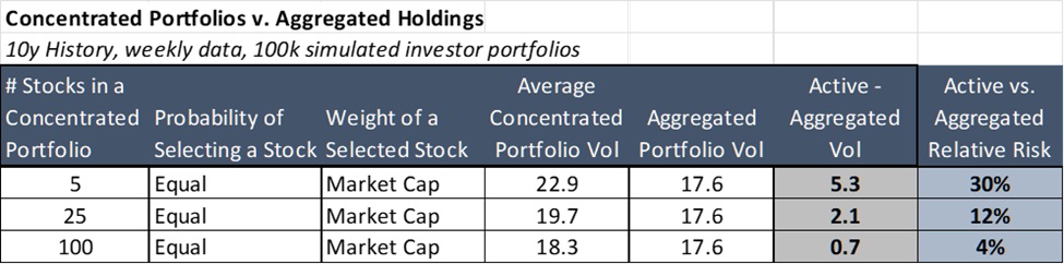
If, as was the case in the 1960s, the median number of stocks in an individual’s brokerage account was just two, the average riskiness of these highly concentrated portfolios would be 1.5x that of the market portfolio. A more recent 2005 study showed that stock investors with liquid assets over $1mm directly hold on average 15 stocks.5
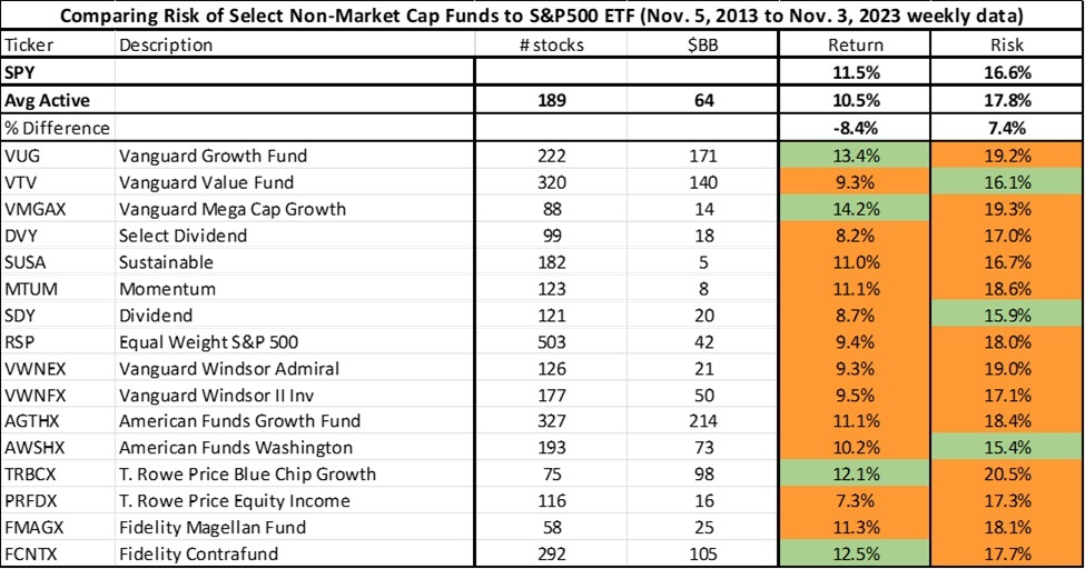
Another viewpoint we can take is to compare the average risk of a set of non-market capitalization-weighted ETFs and mutual funds to the risk of the S&P 500 over the past 10 years. Even though these actively-managed funds hold about 200 stocks each, their average risk was 7% higher than the risk of the relevant market portfolio. In particular, it is very interesting to note that Vanguard’s growth and value funds – which each own over 200 stocks, and represent mirror active portfolios of each other – have an average risk that is 7% higher than the S&P 500.
You might say, what’s the big deal if the risk on a typical actively-managed portfolio is 10% higher than the risk of the market portfolio? Well, we think it is a big deal! Assuming it comprises most of the risky part of a portfolio, to be indifferent between the active portfolio and the market capitalization-indexed portfolio, you’d want them to have the same Sharpe ratio. This means the active portfolio would need to have 10% more expected return net of fees in excess of the safe asset than the market portfolio. If, for example, you think the market portfolio offers a 4% return in excess of the safe asset, then the active portfolio would need to offer 0.4% more, or a 4.4% excess return, just to be equally as attractive on a risk-adjusted basis.6
For years, investors and commentators have bemoaned the roughly 0.6% per annum difference between the average expense ratios on US actively-managed equity mutual funds and US equity index funds.7 We think they should be just as concerned, if not more so, by the extra cost of risk involved in holding concentrated portfolios in aggregate. This cost of risk of active management can easily be as large as or, in extreme cases of concentration, dwarf the extra fees that have garnered investor attention for so long.
Conclusion
Vanguard founder John Bogle was profoundly impacted by Sharpe’s Arithmetic, which he developed into his “Cost Matters Hypothesis” (CMH) presented in the same journal that published Sharpe’s Arithmetic 14 years earlier:8
Gross returns in the financial markets minus the costs of financial intermediation equal the net returns actually delivered to investors…To explain the dire odds that investors face in their quest to beat the market, however, we don’t need the EMH (Efficient Markets Hypothesis); we need only the CMH [Cost Matters Hypothesis]. No matter how efficient or inefficient markets may be, the returns earned by investors as a group must fall short of the market returns by precisely the amount of the aggregate costs they incur. It is the central fact of investing.
In the spirit of the late and great John Bogle, we would like to offer the “Risk Matters Hypothesis” (RMH), as an addition to the EMH and CMH in warning investors of the challenge they face in adding value through stock-picking:
The average risk-adjusted excess return across all active portfolios will be less than the risk-adjusted excess return of the market portfolio, before taking account of fees and trading costs.
As we discuss in more detail in our book, The Missing Billionaires: A Guide to Better Financial Decisions, it is natural that investors should and do require compensation for bearing risk. However, all too often we don’t adequately account for it in our investment decisions.
If there were no extra fees, taxes or other monetary costs associated with active management, Sharpe’s 1991 argument may not have been as influential as it has proved to be. In the past 30 years since Sharpe laid out his arithmetic, there has been a dramatic decrease in the fees charged by active stock managers, commissions for retail stock trades have gone to zero, and the inside bid-ask spread on equities has decreased. Taken together, these have reduced – but not eliminated – the importance of Sharpe’s original argument.
However, in the risk corollary to Sharpe’s Arithmetic described in this note, active investors are engaged in a negative sum activity even if there are no extra fees involved.9 Logic dictates that investors cannot in aggregate be rewarded for the extra risk they incur in owning concentrated stock portfolios.
Using Sharpe’s insightful observation that the portfolios of all active investors must equal the market portfolio and applying it in the dimension of risk, his original warning still rings true that active stock investors in aggregate need to overcome a substantial threshold of extra return in order to improve their welfare.
Further Reading and References
- AQR. (2012). “Why Do Most Investors Choose Concentration Over Leverage?” Alternative Thinking 2Q 2012.
- Black, F. 1986. “Noise”. Journal of Finance 41, 529–543.
- Bogle, J. 2005. “The Relentless Rules of Humble Arithmetic.” Financial Analysts Journal 61 (6), 22-35.
- Bogle, J. 2014. “The Arithmetic of the ‘All-In’ Investment Expenses.” Financial Analyst Journal 70 (1), 1-9.
- Campbell, J. 2018. Financial Decisions and Markets: A Course in Asset Pricing. Princeton University Press.
- Chen, H., Noronha, G. and Singal, V. 2006. “Index Changes and Losses to Index Fund Investors.” Financial Analysts Journal 62 (4), 31–47.
- Dick-Nielsen, J. 2012. “Index Driven Price Pressure in Corporate Bonds.” Working paper, Copenhagen Business School.
- Haghani, V. and White, J. 2023. The Missing Billionaires; A Guide to Better Financial Decisions. Wiley.
- Malkiel, B. 2023. A Random Walk Down Wall Street. W. W. Norton & Company.
- Merton, R. 1969. “Lifetime Portfolio Selection under Uncertainty: The Continuous-Time Case.” The Review of Economics and Statistics 51 (3), 247–57.
- Pedersen, L. 2018. “Sharpening the Arithmetic of Active Management.” Financial Analysts Journal 74 (1), 21-36.
- Sharpe, William F. 1991. “The Arithmetic of Active Management.” Financial Analysts Journal 47 (1), 7–9.
- Stambaugh, RF. 2014. “Presidential Address: Investment Noise and Trends.” The Journal of Finance 69, 1415-1453.
- This not is not an offer or solicitation to invest. Past returns are not indicative of future performance.
We thank John Campbell, Jeffrey Rosenbluth and Mark Grinblatt for their help and encouragement. All errors are our own.
- For discussions of where Sharpe’s Arithmetic may not be a good model of reality, see Pedersen (2018), Chen et al. (2006), or Dick-Nielsen (2012) for the analysis of frictions in bond index funds.
- We recognize this is laid out informally. We hope to come back to this at a later date with a more rigorous treatment, including all assumptions needed. In the same spirit, this result also holds for the average standard deviation of returns, for -1 < ρ < 1, but the math is not as neat and tidy as it is for the average variances.
- We use the past 10 years of weekly return data, and current weights of the Bloomberg 500 US stock index. Our simulated investor portfolios hold stocks with market-cap weights, which is different from the standard calculation of diversification benefits which assumes equal weights, e.g. Malkiel (2023). Once the stock has been selected, we include it with the weight proportional to its market cap. This is because with the equal-weighted approach, it is not possible for the aggregated holdings to match the market weight of the mega-caps like AAPL by aggregating equal-weighted portfolios of more than 15 stocks, since even if each concentrated portfolio holds AAPL (which it wouldn’t), adding them together only gives a 6.7% AAPL weight ( = 1/15) for the aggregated portfolio – below the actual 7% weight. With our approach, an investor holds larger positions in the mega-caps, and therefore needs more stocks to achieve the same risk reduction vs. the standard equal-weighted approach.
- Stambaugh (2014).
- You may also ask, what’s the big deal about a 10% difference in Sharpe ratio, if you don’t expect a higher return on your actively-managed portfolio? The answer is that a 10% lower Sharpe ratio causes a 20% reduction in your risk-adjusted return, as we describe in The Missing Billionaires, Chapter 5, page 59.
- Average Equity and Bond Mutual Fund Expense Ratios Continue to Decline (2022).
- Bogle, J. 2015. “The Relentless Rules of Humble Arithmetic.” Financial Analysts Journal, 61 (6), 22-35.
- Ignoring some possible, though hard to observe or heavily weigh, risk transfer arguments.