By Victor Haghani and Andrew Morton ¹

A thought experiment:

You can invest your wealth in only two assets: a risk-free one and a market portfolio of all public equities. Your investment choices, however, are limited to: A) put 100% in the risk-free asset, or B) 10% in the risk-free asset and 90% in equities. You cannot mix A) and B) – you must choose one or the other. What is the lowest return (above the risk-free rate) you would need to expect from equities for you to choose B? ²

Do you have your number in mind? Great. Now imagine you’re still in this two asset world and you wake up one day and find that the expected return of equities is, in fact, exactly equal to your answer above. But now you’re no longer limited to just options A and B; you’re completely free to invest however much you like in equities, from 0% to 100% or more. How would you invest now?

We’ve asked about a dozen friends this question, all financial professionals. If you’re like them, you’ve likely read the question twice, trying to understand exactly what we’re getting at. You may feel like you just answered that question, and isn’t 90% the answer?

Well, no, we don’t think it is. Please read on as we try to explain why we think 45% is about the right answer, and how we can use the perspective of this problem to answer some other interesting questions.³

You can get an immediate intuition for the problem and its solution by replacing our first question with: how much ketchup on your fries would be so much that you’d be indifferent between no ketchup and that much ketchup? ⁴ And then replace our follow-up question with: how much ketchup is your optimal amount? Our first question was calibrating your risk aversion via indifference points, and the follow-up question involved choosing an optimal point anywhere in between. The halfway point is a pretty good estimate, and exact in some investing models.

Putting a price on risk:

The properties of risk aversion are central to this problem, so let’s analyse the simplest type of risk, a 50/50 coin flip. A side payment is needed to make a typical, risk-averse person indifferent to risking a fraction f of his wealth on such a flip. How should this required side payment vary with f ? There is a very good reason to suggest that it should be proportional to f² , meaning we should demand four times the side payment for twice the risk. To see this, compare a single flip risking √2% of your wealth with two consecutive flips each risking 1%. In both cases the mean and variance of total wealth change are the same (0 and 2).⁵ It seems reasonable that the total side payment should be the same too, which is only the case if the side payment is proportional to f² .

Thus the problem of side payments for coin flips boils down to choosing the specific multiple of f² as your indifference point. Although it’s a matter of individual preference, we suggest a reasonable range for this multiple is 1 to 2.⁶ Let’s use 1, meaning you are indifferent to an offer of 1% compensation to take on a ±10% of wealth flip, or 4% to take on a ±20% flip and so on. You would accept coin flip offers with higher side payments than this, and decline those with lower.

To connect the coin example to the stock market, let’s simplistically model investing 90% of savings in the stock market for one year as risking 18% of wealth on the flip of a coin, meaning over a year we’ll either lose 18% or gain 18%.⁷ The rule suggests that we’d require a side payment of 3.2% (i.e. 0.18²) of our wealth, or 3.6% on the 90% we have invested in equities, to be indifferent.⁸ You can see that in answering the question about what expected return you would need to be indifferent between putting 90% of your savings into equities or 0% in equities, you were calibrating your function of risk aversion.

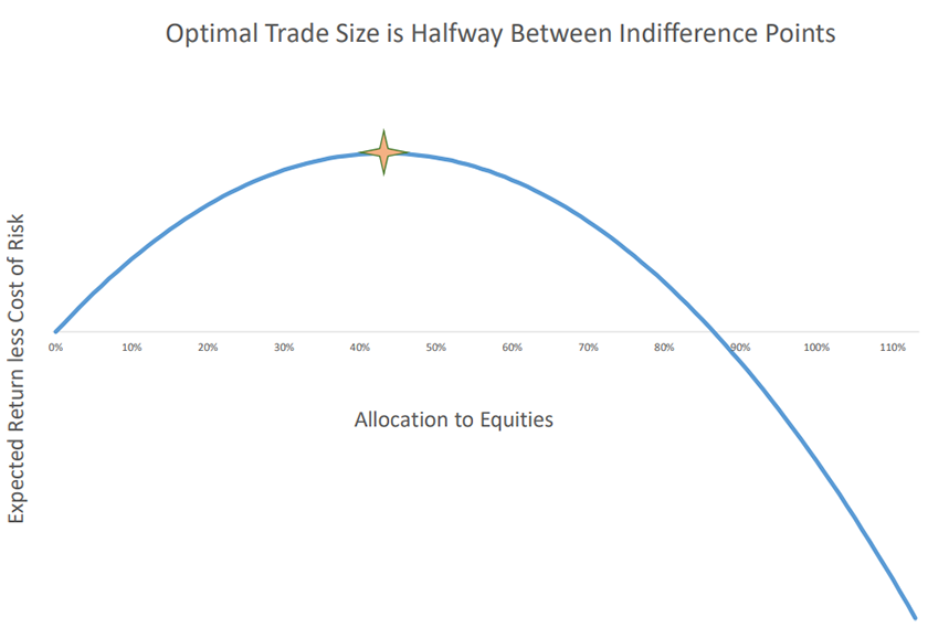
Let’s now turn to the question of how much you should invest given the freedom to choose any trade size you like. Consider what happens as you increase your investment from 0. Your expected gain goes up proportionally, but your risk – and hence, the required reward for bearing it – goes up with the square of the investment. Adding these two effects gives the diagram below, illustrating why the optimal point is halfway between the indifference points of 0% and 90%.⁹ So, someone who is indifferent to investing 90% in equities if they had a 3.6% expected return would optimally invest 45% of his or her wealth in equities at that expected return. In general, optimal size is half the indifference point size.

What kind of questions can we answer with this simple framework?

• What expected return on equities would you need for your optimal allocation to be 75%?
  Recall that the required minimum return you said would make you indifferent to being 90% invested in equities, R_90% , is also the expected return for which 45% is your optimal allocation. Optimal allocation varies in proportion to expected return, and so for it to be 75%, the expected return needs to be 75%/45% higher than your R_90% . For our prototypical investor who has R_90% of 3.6%, the expected return of equities at which a 75% allocation would be optimal is 6%.¹⁰
• What is the effect of over-investing?
  As can be seen from the diagram, if you invest double your optimal allocation, you’ve thrown away all the benefit of the investment, and things get worse at an increasing rate from there. This means we should err on the side of taking less risk in the face of uncertainty about the probabilities of future returns.
• At the other extreme, what about small investments? For example: a $100 coin flip for an investor whose net worth is $100,000?
  The f² rule of thumb suggests being indifferent at a side payment of about (0.001²) x $100,000 = 10 cents! That seems crazy. But if that investor has 45% in the stock market and the rest in the riskless asset, over about one hour his or her wealth will fluctuate by about $100 (with stock volatility of 20%). Using the same 3.6% excess return of equities as earlier, the expected gain in that hour is about 19 cents. So if optimally invested wealth is producing 19 cents for $100 of risk, he or she is roughly indifferent to a side payment of half that. The framework therefore suggests (if needed!) accepting smaller rewards for small risks than might at first seem intuitive.
• Should a passive investor in the stock market have a static allocation to equities?
  Investment advisers typically subject their clients to a risk evaluation to determine an appropriate allocation to equities, often taking the form of the kind of indifference questions we posed. If you believe that the expected return and/or risk of the equity market change over time, then your optimal allocation to equities should also change.¹¹
• Does horizon matter?
  To the extent investments are like coin flips, following a random walk, with the risk we care about (variance) and the compensation we’re being offered to accept that risk both growing proportionately with time, then, whether we choose a month, a year or a decade as the horizon for our investment won’t affect our choice of the optimal amount we should invest in it. Whether we’re flipping a biased coin once or 300 times, the amount we put at risk as a fraction of wealth should be the same.
• How much is it worth to be able to invest in equities?
  We don’t need to believe that we can beat the market for us to put a positive value on the opportunity to invest in equities. Recall that we’re choosing an allocation to equities that maximizes the surplus of what we’re expecting to be paid over what we need to get paid to accept that risk. That surplus is equal to half of the risk premium multiplied by our optimal allocation. So, for example, if we see equities priced to deliver a 5% expected return, and our optimal allocation is 60%, then our surplus is 1⁄2 * 60% * 5% = 1.5% pa . This tidy sum should make us feel pretty good, even grateful, about the existence of the equity market and our ability to freely choose how much of it we’d like. We’re being invited to play a game with favorable odds, like betting on the flip of a coin that has a 60% heads bias, or playing in a poker game where the other players have more money than skill.¹²
• What is ‘Kelly’ betting, and how does it relate? The Kelly criterion, named after the scientist at Bell Labs credited with formulating it in 1956, tells us how to bet to maximize the expected growth rate of our wealth. Implicit in the Kelly criterion is a level of risk aversion that is half of what we’ve been using in these examples. So a Kelly investor in the stock market would need only 1.8% excess return to be indifferent to holding 90% of wealth in the market versus nothing – equivalently, he or she would only need to expect 3.6% to optimally be 90% invested in equities.¹³ This is a much more aggressive posture than most investors we’ve met seem comfortable with.

Conclusion:

We hope this discussion has given you some simple but versatile tools for thinking about a broad range of investment-related questions. Seeing the risk-taking decision more like tuning the dial on a radio, rather than flipping an on-off switch, enables us to get the most out of any game where the odds are in our favor, including investing in the stock market. The trick is to tune your portfolio to the point where the cost of risk, which is increasing quadratically, is just about to grow faster than the expected return you’re being paid to take that risk, which is increasing linearly. We hope you’ve found some ‘utility’ in this brief summary, and that we haven’t taken too many liberties in attempting to distill what are some of the most valuable insights in finance from the last 400 years, from Daniel Bernoulli to Bob Merton, and many brilliant minds in between.

---

Further Reading and References:

• Arrow, Kenneth J. “Alternative Approaches to the Theory of Choice in Risk-Taking Situations,” Econometrica, Oct 1951.
• Bernoulli, Daniel. “Exposition of a New Theory on the Measurement of Risk,” (1738). Translated in Econometrica, (1954).
• Haghani, Victor and Richard Dewey. “Rational Decision-Making under Uncertainty: Observed Betting Patterns on a Biased Coin,” SSRN, 2016.
• Merton, Robert C. “Continuous-Time Finance.” 1990.
• Norstad, John. “An Introduction to Utility Theory,” Norstad.org, 1999.

You can also see our pieces here, here and here on estimating the long-term expected return of the stock market and its risk.

---

1. This not is not an offer or solicitation to invest, nor should this be construed in any way as tax advice. Past returns are not indicative of future performance.
   
2. We will always use ‘the expected return of equities’ to mean the expected return above the risk-free rate.
   
3. If you answered 45%, you can pat yourself on the back and get back to teaching your finance students.
   
4. Sorry, but we’re assuming you’re North American and do like ketchup on your fries.
   
5. To be precise, if the second flip is for stakes of 1% of the new wealth, the variance of wealth change is 2.0001%.
   
6. A multiple of 1 corresponds to that of an investor with power utility function with relative risk aversion parameter n = 2 . The power utility function is given by: u(w) = (w^{1 – n} – 1)/(1 – n) for n ≠ 1 , u(w) = ln(w) for n = 1 . With n = 2 , we won’t accept a fair coin flip where we lose half of our wealth, no matter how big the upside if we win.
   
7. Investing in the stock market isn’t the same as flipping a coin with known probability of outcomes. There is uncertainty in addition to risk concerning the distribution of outcomes. The setup of the problem in this note leaves out many real world practicalities, such as the value of one’s human capital, the correlation of future consumption with the market, and the existence of other assets, to name just a few. We also have modeled the stock market as normally, rather than log-normally, distributed to the one year horizon.
   
8. By the same logic, the risk of the stock market is 18% / 0.9 = 20% .
   
9. The net value for any allocation, k , to equities is: kα f² – k(α f)² , where α is the proportion committed to the risky investment, and k is the coefficient of risk aversion. The objective is maximized with respect to α when α = 1⁄2 .
   
10. Let’s use the notation (P,f) for earning a side payment of fraction P of wealth in exchange for risking fraction f on a fair coin flip. What is the optimal fraction of wealth, k , of this risk we should choose, assuming we are indifferent to flips of (f²,f) ? To be indifferent, we need to choose k such that (kf² = kP , or k = P / f² . The optimal choice is half of that, so  k = 12 P / f² You can see that the optimal allocation, k , moves in proportion to expected return, P , and in inverse proportion to the square of risk, f . So, if stock market risk dropped by 10% (say from 20% to 18% in our example), then your optimal allocation to equities would go up by  1(1 – 10%)²~24%
11. Except if the changes in the return and risk of the market are such as to keep the ratio of return to variance constant.
    
12. We could also view this 1.5% a year as the risk-free payment we’d need to receive to forego being able to invest in the equity market, and only be able to invest in the risk-free asset. We’ve asked a version of this question to about 30 of our friends. We’re still conducting this survey, so stay tuned for the results in a future note.
    
13. As above, assuming 20% annual stock market volatility. The Kelly criterion in continuous time gives an optimal fraction to invest,  f = Rσ² where σ is the annual risk of the stock market.