By Victor Haghani and James White ¹

In a world of low rates and high stock prices, it’s natural that many investors are looking for ways to earn a good return with limited exposure to equities. However, many candidate strategies have return distributions which are significantly different from the Normal and Log-normal distributions that serve as reasonable approximations for the return profile of most typical portfolio asset classes. They require an upgraded set of tools to analyze and incorporate into our portfolio, maintaining a good balance of risk and reward.

As an example, one strategy that we’ve been hearing about a lot recently is buying short-term, high-yielding bonds, particularly financial issues.² On the face of it, this strategy is appealing: these bonds have 4 – 5% yields, seem unlikely to default, and don’t come with a lot of daily market risk. For investors who feel, as many do, that equities are expensive and will generate relatively meagre returns, these bonds appear to provide a lower-risk alternative without sacrificing yield. However, these bonds are quite different animals from the diversified debt/equity portfolios most investors normally think about, and provide an excellent practical illustration of the shortcomings of the most commonly employed investment analysis heuristics.

The first problem is our well-documented tendency, when thinking fast and intuitively, of putting too much weight on highly likely “headline” outcomes and ignoring ones that are very unlikely but extreme.³ We are apt to see the promised return of a 5% bond as the expected return, effectively setting to zero the probability of loss from default. Of course, we know there’s no such thing as a free lunch; 5% bonds can’t be risk-free in a world of 0-1% interest rates. Assuming a 3% probability of losing 65% in a default or restructuring brings the resultant expected return on these bonds to 3%, below the headline yield of 5% but still a healthy 60% of it.⁴

Using the heuristic of expected return, or even the ratio of expected return to risk (aka Sharpe ratio), can lead to a significant mis-evaluation when applied to a case like this. Neither metric gives us an adequate way to weigh the small risk of a large loss, nor do either tell us how much of these bonds we should optimally hold. What’s needed is a more fundamental and versatile tool, a sharper lens for sizing up the proverbial nickels and steamrollers. Expected Utility fits the bill.

It’s a concept that’s been around for a long time, but surprisingly is hardly used by present-day analysts and investors. Tellingly, professional gamblers rely on it heavily (well, those who don’t tend to change profession quickly). It’s the general framework behind the “Kelly Criterion,” a betting and investing guideline used to good effect by Ed Thorp, a pioneer in applying probability theory to gambling and investing, and others such as Warren Buffet and James Simons.⁵

The basic idea is that instead of thinking of our wealth in terms of dollars, we’re going to think in terms of how much our wealth is really worth to us, which we call its utility. For most of us, increasing the dollar value of our wealth delivers less and less utility. A consequence of this decreasing marginal utility of wealth is that we are risk averse: a loss hurts more than the same gain, and we need to be paid to take symmetric risks. Each person’s risk aversion is a matter of individual preference. Starting to think in terms of utility instead of dollar value can be challenging, but we have no choice: to make better decisions we have to get our arms around it.⁶

For the rest of this note, we’re going to assume a level of risk aversion that we think may be typical for high net worth investors. It’s a degree of risk aversion that would leave an investor indifferent between accepting or declining a payment of 4% of wealth in order to take a 50-50 risk of making or losing 20% of wealth.⁷

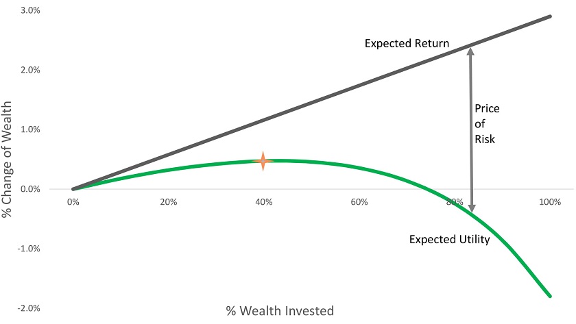
So, coming back to these short-term bonds – what’s the expected utility of owning them? The answer depends on what fraction of our wealth we invest in them. Let’s look at this chart of expected value and expected utility as a function of what fraction of our wealth is invested: ⁸

As you can see, if we put 45% of our wealth into these bonds, we’ve increased our expected utility by the same amount as if we had received a risk-free payment equal to 0.5% of our wealth. A greater or smaller allocation to these bonds is of less utility to us, and beyond a 75% allocation, we’d actually be better off doing nothing at all.

As is clear from the chart, expected utility not only tells us the “price of risk” – the difference between the Expected Return and Expected Utility lines in the chart – but it also allows us to determine how much of the asset is optimal to hold. Even better, we can compare across assets with very different distributions, knowing we’re pricing risk consistently. The heuristics of Expected Return or Sharpe ratio are silent on these critical questions and do not allow for appropriately comparing assets with dramatically different return distributions.⁹ By linking investment inputs and characteristics to optimal size, Expected Utility also gives us an intuitive framework for translating the uncertainty in our assumptions into investment-sizing decisions.

Our analysis so far has been highly stylized, but using this utility framework is a good starting point from which to build in more complex, real-world factors. For example, we could extend the analysis to look at a portfolio of these bonds or the full menu of alternative investments, rather than just a single bond. For taxable investors, we’d want to take account of interest being taxed at high ordinary rates, while the periodic capital losses cannot be offset or carried back. A robust analysis might also bring in other factors such as the timing of potential losses relative to when those losses hurt the most.

To a greater or lesser degree, many popular investment strategies, such as selling puts on the stock market, holding concentrated individual stock portfolios or investing in leveraged hedge fund strategies which don’t or can’t employ tight stop-loss limits, are also good candidates for the application of the Expected Utility framework. Our message here is not that utility is the only thing you need – but rather that for enterprising investors looking at potential investments with highly skewed and/or non-linear return distributions, the standard toolbox of Expected Return and Sharpe Ratio is inadequate. Although Expected Utility analysis is rarely seen in the mainstream, we hope we have illustrated that it is both practical and useful.

---

Appendix: Variation on a Theme

An extension to an interesting and related investment challenge is how to scale a Hedge-fund (HF) investment. In the case of a HF that has an expected excess return of 5% and follows a Brownian random-walk with Sharpe Ratio of 1, then for an investor twice as risk averse as Kelly, expected utility is maximized by investing 1000% of wealth in the HF.¹⁰ This doesn’t pass a basic sanity test, let alone one of prudence! So what’s wrong? Is the utility-corrected lens we’re looking through flawed somehow, or is it that we’re looking at an inaccurate representation of the HF return distribution? We think the lens is fine and that an investment that is fully described by a Brownian random-walk with Sharpe Ratio of 1, with no risk of blow-up, is a truly amazing investment. But, as at least one of your authors can attest, HFs do have a real risk of blow-up with low recovery,¹¹ even if the probability is relatively remote.

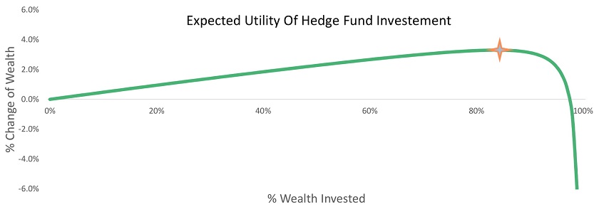
What does our utility framework suggest once we incorporate this tail risk into our analysis? Let’s now assume that most of the time our HF follows the 1-Sharpe random walk as above, but also has a 0.1% / year¹² chance of blowing up with zero recovery. We can see this is just a slightly more complex variation of the short-term bonds example above. As shown in the chart below this blow-up risk, though very small, has a dramatic impact on the optimal scaling recommendation.

Including the small chance of a blow-up yields approximately the same scaling recommendation as for a 0.3-Sharpe Brownian random-walk with a 5% expected return, which is similar to the stock-market. In contrast, including the 0.1%/year chance of blow-up only moves the Sharpe Ratio from 1 to 0.83, a much smaller difference than suggested by the utility framework. Here again, we see that for highly skewed or non-linear return distributions, the toolbox of Expected Return and Sharpe ratio is inadequate, and an expected utility analysis is both useful and intuitive.

---

1. This not is not an offer or solicitation to invest, nor should this be construed in any way as tax advice. Past returns are not indicative of future performance.
   
2. These bonds are usually subordinated or issued at the holding company level, or may even be preferred stock.
   
3. Daniel Kahneman, Thinking Fast and Slow (2010).
   
4. For reference, 3% is the fair-market default rate assuming a 4% equity risk premium and a credit β of 50%.
   
5. See Ed Thorpe’s Beat the Dealer (1966).
   
6. See one of your authors’ notes for more information on calibrating personal utility, available at SSRN: “Practical Utility, Risk Aversion, and Investment Sizing”.
   
7. There are many models for utility, but here we use the most common model   U(x) = x^{1 – n} – 11 – n and assume a typical value of n = 2 for our model investor. In general this leads to betting 50% as much as the “classic” Kelly criterion suggests. This form of utility function is wealth-scale independent.
   
8. Assuming a 5% 1-year bond with default probability 3%, recovery 35%, and a 1% risk-free rate subtracted out so we can just look at excess return.
   
9. Assets with dramatically different distributions can have very different utility and intuitively very different risk profiles, but identical Sharpe ratios.
   
10. Assuming the only investment options are the HF and a riskless bond, and the investment is continuously rebalanced to 1000% of current wealth – generally not a realistic option for HF investments. There’s a classic result that the utility-optimal scaling under these conditions for an asset following a Geometric Brownian random walk is:   κ = μ – rnσ² = 1000% in this case.
    
11. A result of the leverage typically employed.
    
12. Chosen not for perfect accuracy, but to demonstrate the impact of even quite a small blow-up likelihood, in this case 1 HF out of a pool of 1,000 each year.