February 21, 2025
Featured Insights
How Much Insurance is Right For You?
By Victor Haghani and James White1
ESTIMATED READING TIME: 8 min.
Insurance is top of mind for many American families right now, with the dramatic footage and devastation of the Los Angeles wildfires still fresh in our minds, following only shortly on the heels of the watery destruction inflicted on the Gulf Coast by Hurricane Milton. All around the country, those without insurance are likely wondering if they should get it, and those with insurance are bracing for higher premiums and may be contemplating whether it’s cost-effective to keep it.
With so many people we know thinking about insurance, we got to pondering what the right approach is to figure out how much insurance is optimal to carry and how to quantify how much value it’s adding. We looked on the internet and asked our favorite AI engines, and to our surprise, couldn’t find a good insurance calculator that addresses these questions. Longtime readers who know that sizing questions are dear to our hearts won’t be surprised to learn we decided to figure it out for ourselves. Along the way, we discovered a powerful and little-known rule of thumb and built a calculator which is available on our website.
Before we go and flesh out this framework, our intuition is that it should always make sense to fully insure a risk if you can buy insurance at its fair actuarial value, which is to say with no markup above the expected payout from the insurance contract. We’ll discuss why in the next section – but if you’re paying a markup, then there has to be some level at which it makes more sense to partially insure or not insure at all. As an extreme example, imagine if a very large markup caused the premium to be as big as the asset value itself.
The central question we want to address in this note is how to quantify how “price sensitive” insurance buyers should be, and in the context of insurance, what is the “price” they should be sensitive to?
Insurance sizing framework
The canonical paradigm for evaluating financial decisions in the face of uncertainty is the expected utility (EU) framework, which we discuss extensively throughout our research.2 To apply it in this case, we’re going to model the insurance decision for a family with typical risk preferences, and the optimal decision – the ideal amount of insurance to buy – will be that decision which maximizes their expected utility. We can also convert expected utility into certainty-equivalent wealth, allowing us to compare risk-adjusted benefits across different choices.3
We’ve built a calculator around this framework, which we hope you’ll find interesting and useful. We’ll use it for all the exhibits and results below. We’ve also created a spreadsheet that interested readers can use to see the expected utility calculations directly.
Let’s start with a family with $1 million of wealth, including the value of their home, and a risk-aversion coefficient of 3, within the range of typical levels but on the conservative side.4 They’re looking at insuring their house, which has a replacement cost of $800k. There’s a 0.5% chance every year of the house being destroyed, and they can fully insure it for $4,000 per annum – the actuarially fair rate. For this example, we’re making the unrealistic assumption that the insurance company is not charging any markup at all above the expected payout of this insurance policy. The chart below shows the difference in risk-adjusted wealth, expressed as a percentage of total family wealth of $1million, between not insuring and insuring a given amount of the house for one year.5
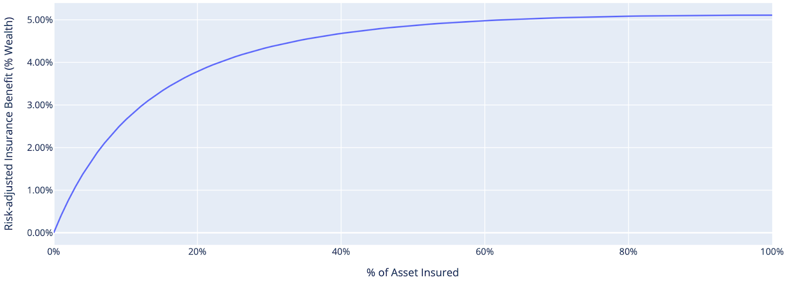
As we expected, in this case, it’s optimal to fully insure. Doing so adds tremendous value, equivalent to about 5% of total wealth – and that’s just for one year! If we run these same calculations for different degrees of risk-aversion, probabilities of loss and fractions of wealth in the house, we’ll see that the EU framework confirms our intuition that if you can insure at the actually fair rate, it’s always optimal to fully insure.
The reason why is that insuring at fair rates, by definition, neither increases nor decreases your expected wealth – it has 0 expected return – but it does decrease your risk. This should always be a good thing, and in our framework, it will always formally increase your expected utility. So, given fair insurance for a risk you’re bearing, you should always take as much as you can get, up to the amount of the risk you’re insuring.6
Here we can see why insurance – if priced reasonably – is one finance’s most valuable contributions to society. By leveraging the power of risk pooling, individuals can secure peace of mind, protect themselves against catastrophic losses, and very significantly increase their individual and collective risk-adjusted wealth.
Alas, free lunches are hard to find
Of course, it’s not easy to find actuarially-fair insurance! Insurance companies have to set prices high enough to cover not just expected payouts, but also brokerage commissions, administrative costs, allowances for some fraudulent claims, and a profit margin on their capital.
We’ll call this markup in insurance policy pricing the “insurance premium margin,” and we’ll define it as the fraction of the premium remaining after the expected payout. If you have a home insurance policy which costs $5,000 per year, and you think that the actuarially fair value of that policy is $3,500, then:
\[\textit{Insurance premium margin} = 30\% = \frac{5,000 – 3,500}{5,000}\]
At this point, you’re probably wondering how you can figure out the “actuarially fair” value of an insurance policy you’re interested in. Unfortunately, insurance brokers – who typically receive commissions of 10-20% – don’t tell us this information, nor do the insurance companies or the insurance regulators. For some insurance products like life insurance (insuring against dying early) and annuities (insuring against dying late), actuarial mortality tables are publicly available and sufficiently accurate.7 For home and auto policies, based on discussions with several insurance industry experts and from whatever public information we could find, it seems that the margin is around 30% for policies of $5,000 or more per annum, and the margin is higher for policies involving smaller premiums.
Of course, the margin can vary dramatically, and there are even situations where insurance policies are priced below the expected payout. These cases usually arise as a result of government regulation putting caps on insurance premiums, which insurance companies accept in order to conduct other more profitable business in that jurisdiction.
We should be sensitive to margin, rather than premium
Assuming there aren’t direct cashflow constraints, insurance buyers should be sensitive to premium margin, not the raw premium amount. A recent WSJ article titled “The World Is Getting Riskier. Americans Don’t Want to Pay for It” suggests that people tend to reduce the insurance they buy when the raw premium goes up. But we believe – as we’ll show below – that people should reduce their insurance only if the margin increases, not if the raw premium increases because the risk of loss has risen.8 In fact, buying insurance gives you greater risk-adjusted benefit when the risk of loss goes up, as long as the margin in your policy remains constant.
But how margin-sensitive should you be?9 Let’s come back to our case of a family with $1mm of wealth, 80% of which is a home they want to insure. Below we see the increase in risk-adjusted wealth from insuring the home to different levels, where each line represents a different margin charged by the insurance company.
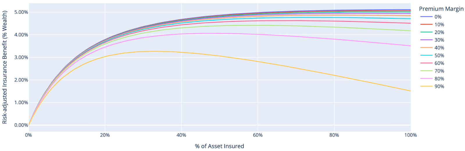
We can see that, given our assumptions in this case, fully insuring is either optimal, or so close to optimal as to make no difference, up to about a 60% margin. As the margin increases from there, fully insuring still adds risk-adjusted benefit, but becomes increasingly sub-optimal as the margin you’re paying increasingly outweighs the core risk benefits of the insurance. A 90% margin means the premium is ten times higher than its expected value, and In that case, the optimal amount to insure for this family is just 30% of the value of their home. It’s not hard to see how such a big margin makes the insurance contract sufficiently less attractive that you shouldn’t want much of it.
Risks come in all sizes
So far, we’ve primarily been looking at the case of insuring an asset which is a large fraction of net worth. What about insuring smaller risks? Let’s turn to the case of a family with $5mm of wealth and a $1mm home, with the same risk preferences as before:
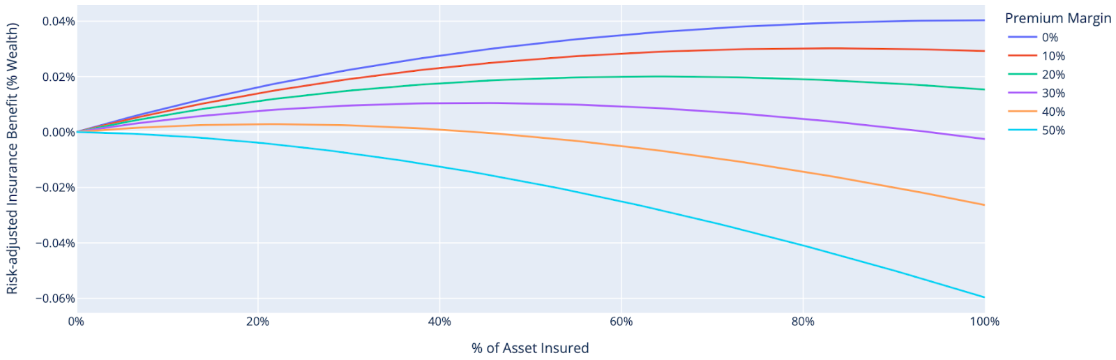
The first thing we notice is the remarkable difference in scale. With the insured house worth 80% of wealth, insuring was incredibly consequential, delivering a risk-adjusted benefit on the order of 5% of wealth – but with a house worth 20% of wealth, even with no premium margin at all, the maximum risk-adjusted benefit is more like 0.04% of wealth. This is because, for a given amount of risk-aversion, there’s less asymmetry between positive and negative outcomes over smaller and smaller changes in wealth.10
Given the dramatically lower expected benefit, it’s perhaps not surprising that increasing margin reduces the optimal insurance level more quickly than in the previous case. For a 30% margin, we can see the optimal amount to insure is around 40%. The difference between optimally insuring and fully insuring is small relative to wealth, but we see that fully insuring is actually (very slightly) worse than not insuring at all, and a considerable difference relative to the maximum benefit. At a 50% margin, you optimally wouldn’t insure any amount at all – that is to say you’d fully self-insure your home. For a low probability of a 20% loss in wealth, paying the margin eats up all the risk benefits of the insurance.
The Campbell-Ramadorai (CR) rule of thumb11
Rather than using our insurance calculator, here’s a rule of thumb that gets remarkably close to the full expected utility analysis: you should insure an amount of your at-risk asset such that if the loss occurs, your drop in wealth will be equal to the premium margin divided by your coefficient of risk-aversion.12
For example, if the insurance you’re considering has a 30% margin13 and your coefficient of risk aversion is 3, you should buy enough insurance so that a loss results in your wealth falling by 30% / 3 = 10%. So, if your home represents 20% of your wealth, you should insure half of it, as we found in our base case above. If your home represents 10%, or less, of your wealth, you should optimally insure none of it given a 30% margin.
It’s really quite remarkable that, to a first-order approximation, only two things matter in your insurance decision: the margin embedded in the policy and your level of risk-aversion.
Small risks
For most people, the risk that your dishwasher breaks is a minor risk in relation to wealth, and doesn’t make sense to insure if you believe there is any margin built into the policy premium. In fact, it’s likely that insurance policies on small risks like appliances will have larger margins, since insurance companies will tend to incur administration costs that are large in relation to the value of the item being insured.
An interesting case that tends to be in between home insurance and a dishwasher warranty is the choice to go for comprehensive in addition to third party liability car insurance. Here, you’re paying extra to buy insurance against your car being damaged, destroyed or stolen. For many people who own their cars outright without debt, the loss of a car will represent less than 10% of wealth. With a 30% insurance premium margin or higher, it’ll make sense to self insure fully against that risk. Even if an individual is extremely risk averse, it’s unlikely that insuring a risk that will result in less than a 10% loss of wealth will be worth the cost.
Bundling of big and small risks
Insurance companies often offer policies that bundle big and small risks together. This is typically the case in home insurance, where your home will be covered against total loss – but at the same time, you’ll be covered against minor damage, like frozen pipes or a leaky roof. Given that insuring small risks usually isn’t a good idea, it follows that the forced bundling will make you want to buy less insurance overall than if you can buy your insurance only on the most consequential hazard. If your insurance carrier won’t unbundle, the use of a higher deductible can effectively take the smaller hazards out of your policy.
Moral hazard
While partial insurance – through insuring less of an asset or accepting a high deductible on the coverage – is the optimal decision whenever an insurance policy is priced at a premium to its actuarial value, there are additional reasons it can be more attractive than full insurance.
Moral hazard refers to the increased likelihood of risky or careless behavior by policyholders after they obtain insurance, knowing that the insurer will cover potential losses. Two common examples are neglecting home maintenance in the knowledge that if significant damage occurs the insurer will cover repairs, or increased risk-taking in driving knowing the insurance company will cover repairs to your car. Insurance companies are acutely aware of the moral hazard phenomenon, and will usually price policies with large deductibles, or partial coverage, more attractively, that is, with a lower markup, knowing such structures reduce the incentives for bad behavior.
Other insurable risks
There are a number of types of insurance which are more complex than the property insurance examples we have discussed so far. These include medical, long-term care, life and umbrella liability insurance. In these cases, we also believe that the expected utility framework can be useful in making sound decisions, but a discussion of the framing of these problems is beyond the scope of this article. One of these more complex risks we have written about is the insurance of longevity risk with annuities: The Annuity Puzzle: How Big is the Free Lunch Being Left on the Table?
Financial market insurance
If fully insuring a house always makes sense if you can do so with no margin, what about your stock portfolio? The same logic holds here, if you could insure your portfolio at an actuarially-fair level you always should do so – but in this case, market efficiency tends to conspire against us, and we should expect that insuring against systematic market risks will always carry a margin.14 We explore this question in greater detail in “What About Options?” (chapter 16) of The Missing Billionaires, and find that using put options as portfolio insurance rarely makes sense.
Conclusion
We’ve seen cases where the insurance decision is hugely consequential and others where it’s pretty marginal. In our normal lives, most of us are faced with many opportunities to buy insurance, from smaller hazards such as AppleCare iPhone screen protection, warranties on appliances, and pet insurance, to bigger-but-not-catastrophic risks such as comprehensive car coverage and art insurance. While many of these decisions may not be individually important, making good decisions on the many insurance decisions that you face can add up to a more significant sum over multiple hazards over a lifetime.
Sometimes, our intuition leads us astray – for example, when we’re tempted to reduce coverage when the insurance premium goes up due to increased risk of loss rather than an increase in the margin charged by the insurance company. Even if you feel the net benefit from making the right decision on insurance is inconsequential in your overall financial affairs, we hope that you’ll feel more comfortable and confident having access to a framework and a simple tool for making these decisions thoughtfully.
The insurance decision is primarily a function of the size of the hazard relative to a family’s total wealth, the family’s risk-aversion, and the margin in the insurance policy being considered. Families can readily figure out the first two inputs to their decision, but they are ill-equipped to determine the degree of margin. We hope that this note increases awareness of the central role of margin in the insurance decision, and encourages insurance companies, brokers and regulators to provide greater disclosure of the insurance premium margins embedded in different policies. This will help families make more informed decisions on how much insurance to buy, and could generate a huge aggregate gain in societal welfare.
Building intuition for deciding on low probability, high consequence gambles

Losing 20% of your wealth is a lot better than losing 80%, but it still feels like a very consequential loss. Our expected utility analysis finds that if the insurance premium margin was 50%, your home represents 20% of your wealth, then the optimal decision is to completely forego insurance on your home.15 Can it really make sense to not insure a 20% loss in order to save a small amount of insurance premium margin?
Let’s try to build some intuition for this decision without using an expected utility calculation. We’ll assume that the probability of total loss of your home is 0.2% per year, and the insurance premium you’d have to pay equals 0.4% of the value of your home. The insurance premium margin in this case is therefore 50%.
The above insurance decision is equivalent to asking whether you would take the following gamble: an urn is filled with 1,000 balls. Two of the balls are black, and the other 998 are white. You reach in and pull out a ball. If it’s white, you get a payment equal to 0.08% of your wealth. If you pick one of the two black balls, you lose 20% of your wealth. Your expected payout
(\(\frac{998}{1000} x 0.08\% = 0.08\% \)) is twice as big as your expected loss (\(\frac{2}{1000} x 20\% = 0.04\%\)).
We suspect many people would be disinclined to play this game as it feels like the proverbial picking up pennies in front of a steamroller.16 We think it’s a really difficult decision to make based on gut feel alone17 – but not all gambles are so challenging to evaluate. Assessing the attractiveness of favorable 50/50 gambles is easier than deciding on favorable ones involving a very low probability of a large loss, like the typical insurance decision, and our urn game. Isn’t it easier to decide whether you’d take this gamble: would you be willing to flip a fair coin, where your wealth increases by 20% if you flip heads, but decreases by 10% if tails?
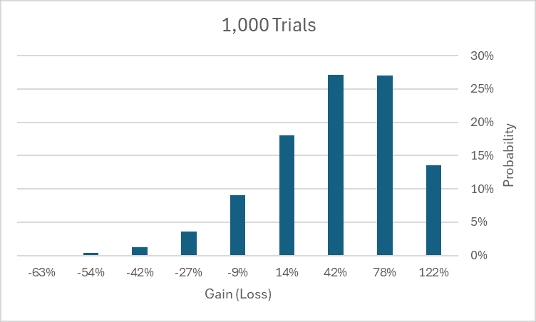
One perspective you could take that might help you decide whether to take the urn gamble would be to imagine you could play the game many times (always replacing the ball you chose and giving the urn a shake), until you started to see a distribution of outcomes that looked more symmetric. For example, if you could play the game 1,000 times, you’d expect your wealth to grow by 50%, with an 85% chance of making a profit, and a 1/1000 chance of losing more than 50%. The chart below shows the probabilities of profit and loss outcomes.18 We’d guess that you’d find playing the game sequentially 1,000 times an attractive proposition, but you might object that just because you’d be willing to play it 1,000 times doesn’t mean you’d be willing to play it just once.19
Here’s another way to think about the gamble that might make the decision easier to make. Your probability of choosing a black ball is 0.2%. That is almost exactly the probability of flipping tails nine times in a row with a fair coin.20 We can design a game involving flipping a fair coin that is equivalent to the pick-a-ball-out-of-the-urn gamble.
The table below shows a series of nine bets, where if you lose all nine in a row by flipping tails nine times consecutively, you’ll lose 20% of your wealth – but if you flip heads just once, you get a payment equal to 0.08% of your wealth and the game stops. Let’s start by focusing on the 9th bet, where your wealth goes up by 15% if you flip heads, or down 8% if you flip tails. We think most people would be happy to take that bet. Maybe the bet before that – win about 9% versus lose about 6% – also feels pretty good.
| if Heads wins | if Tails wins | |
| 1st flip | 0.0800% | -0.0797% |
| 2nd | 0.160% | -0.159% |
| 3rd | 0.319% | -0.313% |
| 4th | 0.63% | -0.61% |
| 5th | 1.25% | -1.17% |
| 6th | 2.45% | -2.14% |
| 7th | 4.7% | -3.7% |
| 8th | 8.7% | -5.7% |
| 9th | 15.2% | -7.9% |
We chose the bets in the table to all be ones that a person with a typical degree of risk-aversion would be happy to take. However, we suspect that as you work your way up the table, you’ll start to wonder whether you should take those bets – particularly the first bet, which seems extremely close to even-money. The thing to remember is that the compensation needed for taking smaller gambles goes down with the square of the size of the gamble. For example, you should require just ¼ the compensation to take a gamble ½ the size of a larger one. Flipping a coin four times, each time to make or lose $1, is about the same risk as flipping a coin once for a $2 gamble.
We hope these alternatives perspectives presented here in this light blue box make sure you don’t see our EU calculations as being in a black box.
Appendix: Campbell-Ramadorai Rule of Thumb Derivation
Man of the best rules of thumb can be arrived at from multiple directions, and this one is no exception. Our derivation is not the original as the namesakes have described to us, but we think this one requires somewhat less background and is in a similar spirit.
As a local approximation to CRRA utility, we assume CARA utility:21
\(u(w) = -e^{-\gamma w}\)
Then assuming a starting wealth of \(1\), as asset to insure worth \(\alpha\), insurance premium of \(\pi * \alpha\), probability of loss \(1 – p\), and fraction to insure \(k\), we have:
\(E[u] = p u\left(1-\kappa\pi\alpha\right) + (1-p) u(1 + \kappa\alpha – \alpha – \kappa\pi\alpha)\)
Using the standard procedure to maximize \(E[u]\) wrt \(\kappa\), we have:
\(\frac{\partial E[u]}{\partial \kappa} = \alpha\gamma\left( (\pi-1)(p-1)e^{\gamma (\alpha+\alpha\kappa (\pi -1)-1)} -p \pi e^{\gamma(\alpha\kappa\pi – 1)}\right) = 0\)
therefore, after some algebra:
\(\kappa^* = 1 + \frac{ln\left(\frac{(\pi-1)(p-1)}{\pi p}\right)}{\alpha\gamma}\)
Now, we introduce the premium margin \(m\) as:
\(m = \frac{\pi – (1-p)}{\pi}\)
or:
\(\pi = \frac{1-p}{1-m}\)
Substituting this expression for \(\pi\) into \((4)\), we have:
\(\kappa^* = 1 + \frac{ln\left(1-\frac{m}{p} \right)}{\alpha\gamma}\)
We define the wealth fraction lost if the optimally-sized insurance pays out as:
\(\lambda^* = (1-\kappa^*)\alpha = -\frac{ln\left( 1-\frac{m}{p} \right)}{\gamma}\)
Now we make two approximations: \(p \approx 1\), and \(ln(1 – x) \approx -x\), yielding:
\(\lambda^* \approx \frac{m}{\gamma}\)
Further Reading & References
- Arrow, K. (1974). “Optimal insurance and generalized deductibles.” Scandinavian Actuarial Journal 1: 1-42.
- Campbell, J. and Ramadorai, T. (2025). Fixed: Why Personal Finance is Broken and How to Make it Work for Everyone. Princeton University.
- Haghani, V. and White, J. (2023). The Missing Billionaires: A Guide to Better Financial Decisions. Wiley.
- Haghani, V. and White, J. (2025). “Buying a Dream, Losing a Future: The Financial Fallacy of Lottery Tickets for Low-Income Households.” Elm Wealth.
- Haghani, V., Ragulin, R. and White, J. (2022). “Do Options Belong in the Portfolios of Individual Investors?” The Journal of Derivatives.
- Ip, G. (2025). “The World is Getting Riskier. Americans Don’t Want to Pay for It.” The Wall Street Journal.
- This is not an offer or solicitation to invest, nor are we tax experts and nothing herein should be construed as tax advice. Past returns are not indicative of future performance. Thank you to Professors John Campbell and Tarun Ramadorai for giving us the inspiration and direction to write this article. Thank you to Dave Blob, Rich Dewey, Mimi Duff, Mark Haghani, Sassan Mikhtchi, Bill Montgomery, Vlad Ragulin and Jeff Rosenbluth for your valuable comments and suggestions, and a special thank you for a set of very extensive comments and corrections from Larry Hilibrand. Of course, all remaining errors are our own. Finally, we appreciate the help of our colleagues Jerry Bell and Steven Schneider who are consistently instrumental in getting our articles to our readers.
- Some would say our book, The Missing Billionaires: A Guide to Better Financial Decisions, speaks of nothing but Expected Utility.
- See The Missing Billionaires Chapter 5: The Mechanics of Choice.
- Assuming CRRA risk aversion.
- We recognize that insurance policies usually don’t allow the buyer full flexibility to choose exactly how much of an asset he wants to insure, but we’ll discuss the insurance decision as if it is possible to make that choice. Often, it’s possible to effectively partially insure through the choice of the policy deductible.
- If you take more, you start to add rather than reduce risk.
- Though it usually is worthwhile to make adjustments for known health and lifestyle circumstances.
- This simple result holds pretty tightly even up to a 10% probability of loss per year.
- For homes with mortgages, fully insuring is typically required.
- This is the case with the standard types of utility curves most often used to represent individual risk preferences, such as constant relative risk-aversion utility curves.
- Thank you to Professors John Campbell and Tarun Ramadorai for sharing this rule of thumb in their forthcoming book: Fixed: Why Personal Finance is Broken and How to Make it Work for Everyone, Princeton Press. We love rules of thumb in finance, and we particularly like ones like this that are both easy to remember and extremely useful!
- Readers may wonder whether the Merton share could also be used as a rule of thumb for the insurance decision. No, it is not a good rule of thumb in this case. Its assumptions are so divergent from the insurance setting that it will give answers far wide of the mark.
- The rule of thumb is more accurate if you measure markup as the natural log of the cost of the insurance divided by the actuarial value of the insurance, rather than the simple ratio we used earlier.
- Specifically, “actuarially fair” in this case means being able to buy downside state claims at the real-world probabilities. But the risk-neutral state prices will always be higher than the real-world fair prices for any asset with a positive risk premium.
- We’re still assuming risk aversion of 3. This is a case where the CR rule of thumb is off by a bit. It would suggest insuring one-sixth of the value of your home, but the EU optimal is to insure none of it.
- Or, after pennies are no longer minted, it’ll be like picking up nickels in front of a steamroller.
- Nor do we think it’s much help to state that the expected return, risk and Sharpe ratio of this gamble are 0.04%, 0.9% and 0.044 respectively. Applying the Kelly criterion to the urn gamble presented here would conclude that yes, the gamble should be taken. In fact, optimally, the gamble should be taken for a downside of 40% of wealth versus a gain of 0.16% of wealth, i.e. twice as big a risk as the game being offered. Such a result is perhaps an illustration of why many risk-takers feel that Kelly assumes an unrealistic degree of risk-tolerance.
- There is some probability mass to the left of -63%, but we cut the chart there because it is not visible to the naked eye.
- This is a hotly debated argument. See Paul Samuelson, A Fallacy of Large Numbers (1963) for a starting point on the debate.
- The exact probability is 1/29 = 1/512 = 0.1953%.
- This approximation will make the marginal utility expression more analytically tractable.