H1 2024 Investor Call Q&A with Victor & James
By Victor Haghani and James White
Thank you to all our Elm investors who joined us for our first investor call of 2024. If you’d like to watch or listen to the full recordings, you can find them here:
Elm Investor Calls
James White:
So, we wanted to start just by through an overview of 2023. I thought a fun thing to do that we haven’t done on this call before would be, rather than showing slides in the presentation, to show the actual tools that we use ourselves and are available to clients.
This is our Asset Allocation tool:
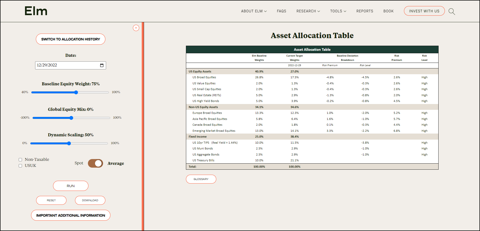
It’s available to not just all clients, but all people in the world. You can go to our website and it’s just Tools, Allocation Viewer. There are two panes to it: the default pane, which allows you to look at asset allocation details on one particular day. Then, you can also switch to Allocation History and put in any start date and end date, your dial settings, and look at what the history of asset allocations is over that period.
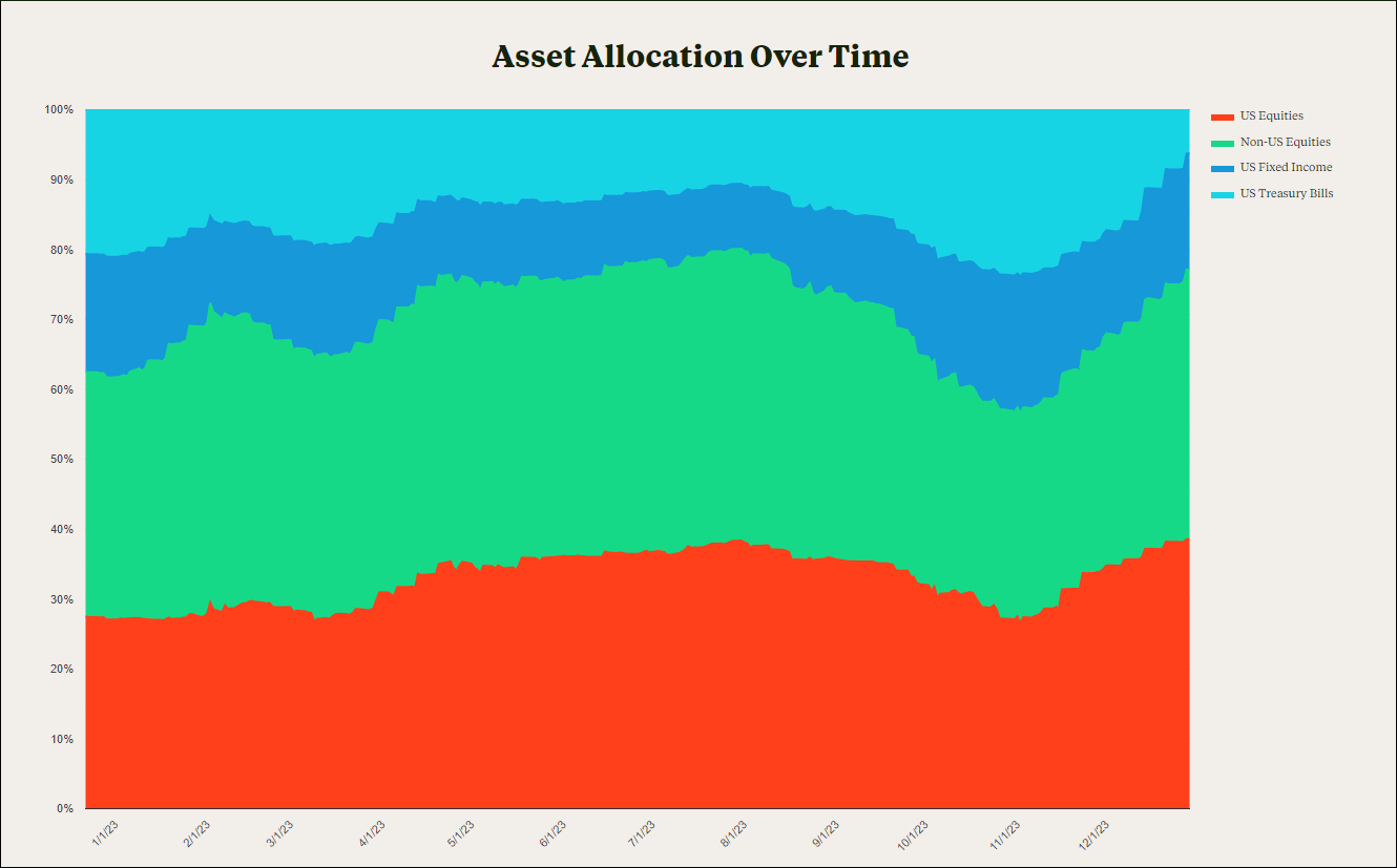
This is all model data of course, and you can go back to 1975 – within the next month or so, we’re planning on pushing it back to 1900 (we actually have all of the data and everything run already, we just need to get a little bit faster in the tool itself). For the history, with the details off, we divide it into the red (which is US equities), the green (which is non-US equities), the blue (which is duration-fixed income), and the light blue (which is short-term fixed income or treasury bills):
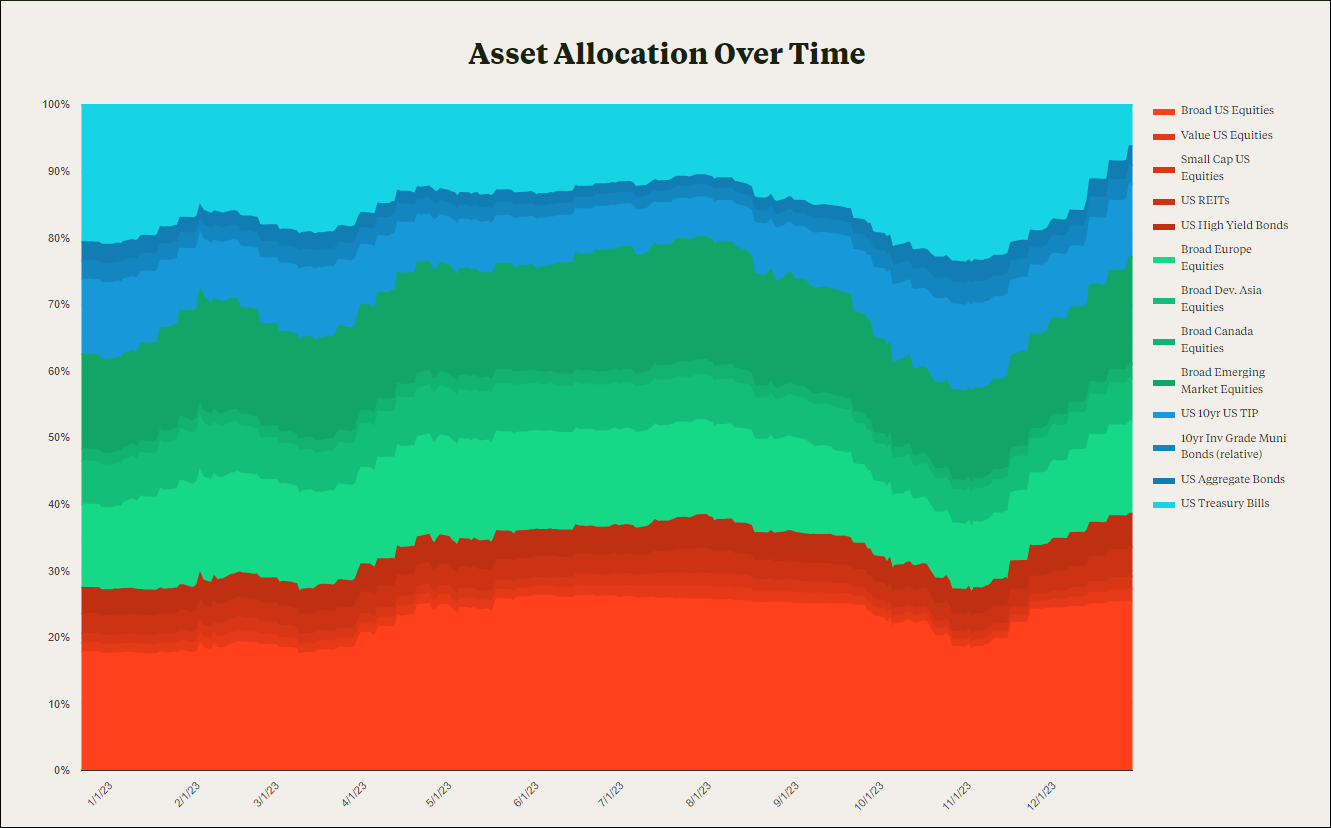
Then, you can click the ‘Detail’ view and see the finer grain, dividing up amongst all of our all of our asset buckets. I’m going to run this now with a baseline of 75% equities, default global mix, and 100% dynamic scaling – but obviously, you can run it with any dial settings, whatever is appropriate or whatever you have or want for your account.
So, relative to a 75 baseline, we started 2023 at about 50% equities – reasonably underweight. By June, we were back to about neutral. Then in September, there was this big drop down to 40% equities, and then we finished the year at about neutral again. What was going on here?
We went in underweight because, coming out of 2022, momentum was negative, risk was high in pretty much every global equity market, and US risk premia were pretty tight. Then, over the first three to four months of the year, momentum flipped from negative to positive: first in the US, and then across the board. Then in September, there was this huge market swoon where momentum flipped negative and then the market staged this tremendous rally in the last six weeks of the year; momentum flipped back to positive. So, this transition from neutral to underweight and back to neutral was really driven by momentum – and if you want to get into the details of that and see what was really going on at any particular date? You can switch to the table view.
The first column shows what the baseline is, and the second column shows the target weight as of this date. You can see that, as of the end of ’22, we were significantly underwent US equities, we were pretty neutral with non-US equities, and we were overweight fixed income. Where is that coming from? Well, looking at US equities, we breakdown the deviation from the baseline into risk premia and risk level. Then, in the last two columns, we show what the risk premia are and what the risk level is.
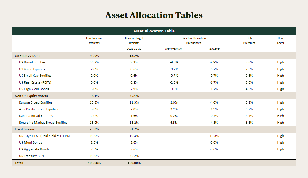
So, you can see that across the board in US equities (with the exception of high yield bonds), risk premia are quite low. 2%, 2 ½% risk is high. That results in the US being underweight both on a risk premium and a risk level basis. In contrast, for non-US equities, risk premia are pretty high, but the risk level is high too. We’re kind of overweight from risk premia, but underweight from risk level, and those things offset each other. And, if you want to see what changed over the year, you can put in 2023 instead.
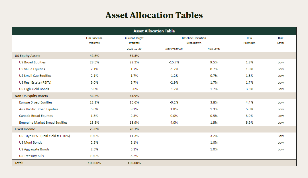
So what changed? From the beginning of ’23 to the end of ’23, the risk level went from high to low, momentum flipped from negative to positive in every major equity market, US risk premia are even lower than they were at the beginning of the year – they started at 2.2-ish, and now they’re 1.8-ish – and non-US equity risk premia are slightly lower as well.
These two tools are the main tools that we ourselves use to understand what’s going on with Elm’s asset allocation, and they’re available for our clients to use as well. For more information about what all the columns mean, there’s a glossary here that defines everything – and, several times in this call, I’m going to plug our new white paper. We have a new white paper, a link was included in our latest quarterly letter – if you can’t find it, feel free to ask us for it anytime. We think that even longtime investors will find it useful and interesting, and we encourage everyone to read it. There’s a lot more definition about what is going on in there, as well as in the glossary.
There’s another tool which is available to all of our investors: the Returns Tool. It is not on our public website – for regulatory reasons, we can’t have it on the public website, but we include links to it in the quarterly letter. It’s basically the same as the Asset Allocation tool, but shows the returns associated with those asset allocations. I’m going to run it for ’23 with one specific set of dials – but you can run it with any dials, and you can also download the data.
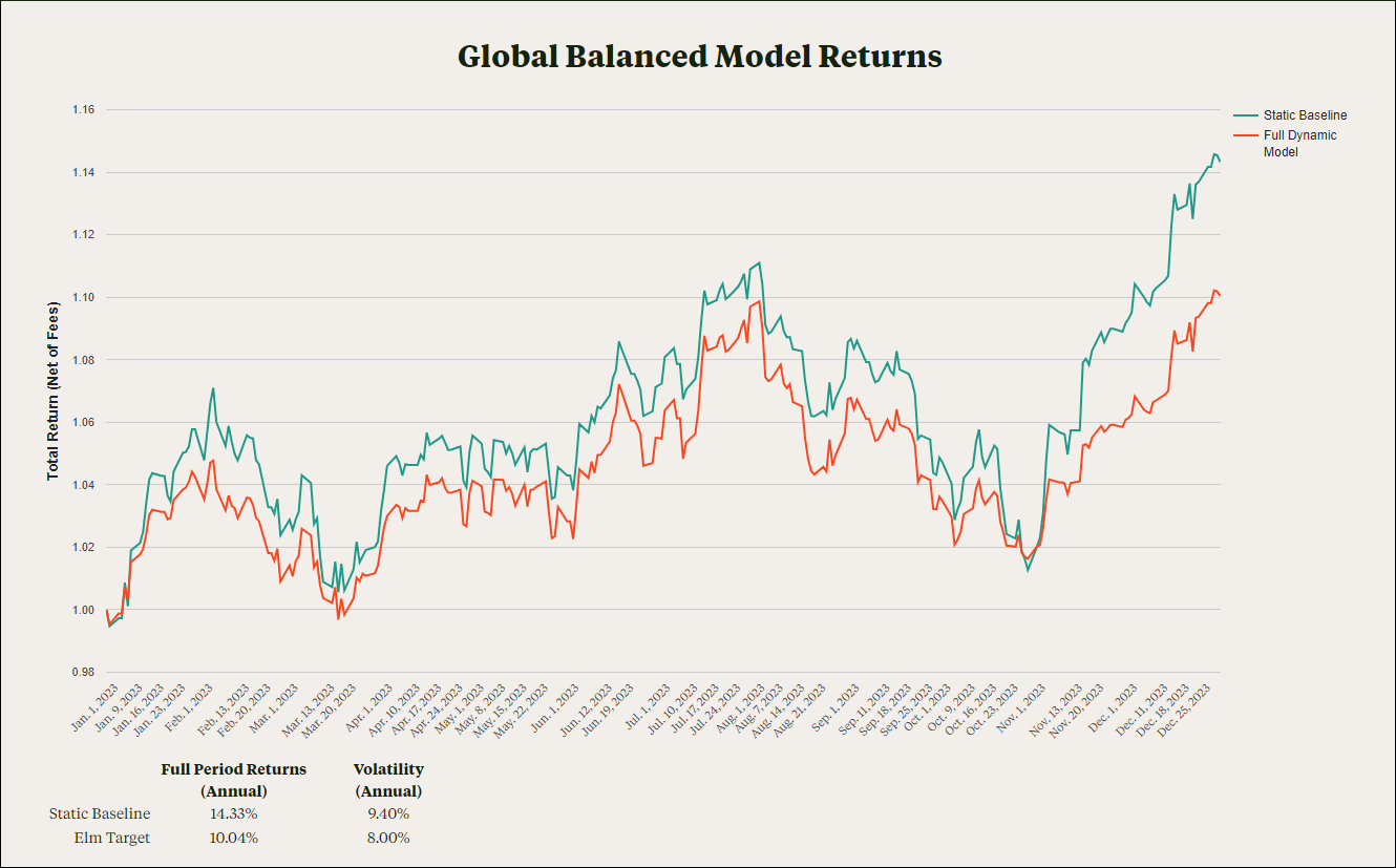
This was returns over ’23. The green line is the static baseline, which, in this case is 75% global equities, 25% cash and bonds. The orange line is the dynamic model. It was a wild year: from January through November, we were basically flat to the model, and then the last two months of the year were really bad. We significantly underperformed, and that led to the model’s significant underperformance over the course of the year relative to the baseline.
On a human and emotional level, whenever Elm is outperforming, we never like to see it. On an intellectual level, we try to be more cold about it. We know that, given the Sharpe ratios involved, there’s going to be plenty of years where we outperform, there’s going to be plenty of years where we underperform. We try to be good Bayesians where we start with our prior – we have a pretty strong prior about the benefits of dynamic asset allocation in this way, which is both theoretical and empirically derived. And when new data comes in – every year, whether we outperform or underperform – we ask ourselves, given the new information, “How much should we update our prior?”
For example, if we expect that one standard deviation of annual outperformance or underperformance is going to be 6%, and then in a given year, we outperform or underperform by 3% – that doesn’t give us a lot of information about updating our prior. On the other hand, if we expect 6% standard deviation and we get a 20% event – that really tells you a lot, that’s going to significantly affect our prior, that’s something really unexpected. So how does this year’s underperformance fit into that?
This shows one particular dial setting for 75% equity, default global mix and 100% dynamic:
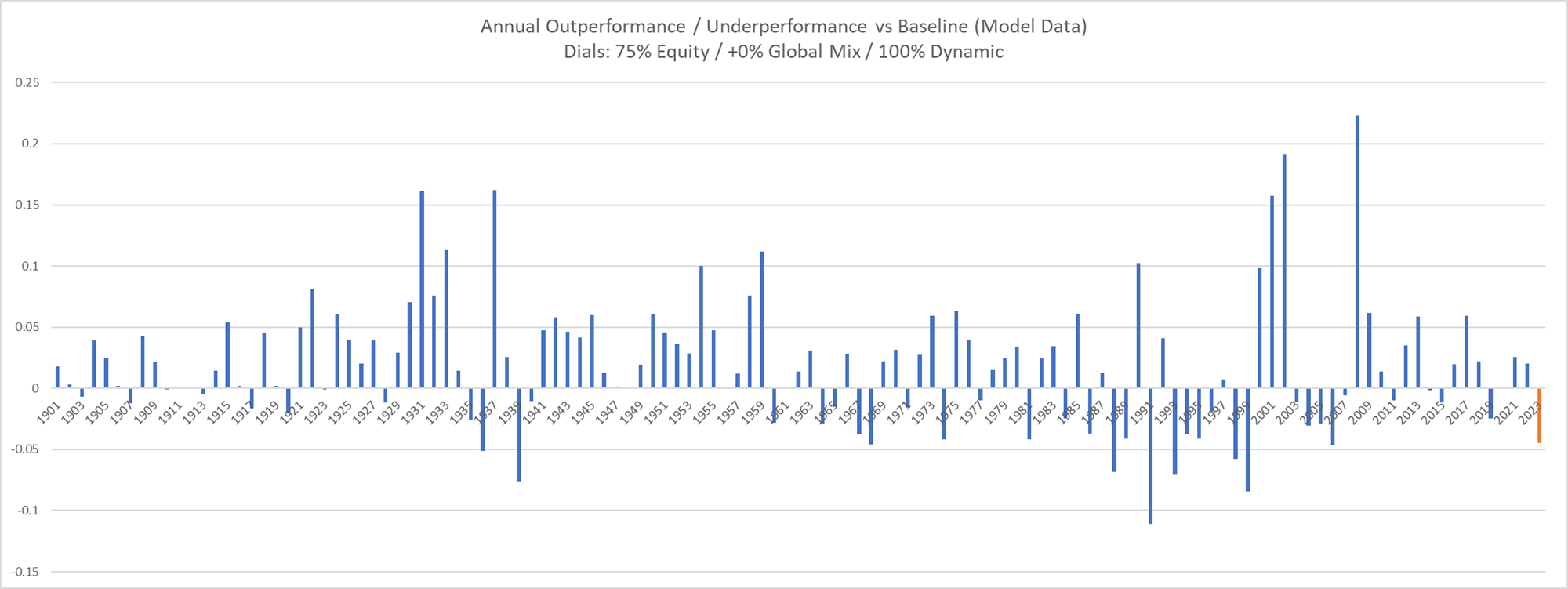
Elm’s model outperformance or underperformance versus baseline since 1900. As you can see, plenty of years of outperformance, plenty of years of underperformance – 2023 is right here at the end, and the circle is basically Elm since inception. This was the largest year of underperformance since Elm’s inception – but over a larger historical context, by no means the largest or a particularly unexpected amount of underperformance.
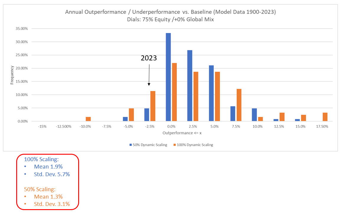
This shows, for 100% scaling and for 50% scaling, the distribution of annual outperformance/underperformance over the last 120+ years:
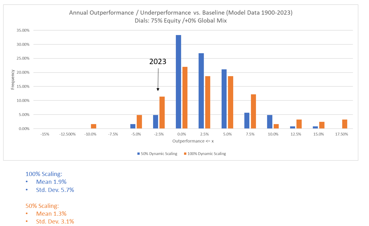
For 100% scaling, the mean outperformance was about 2%, but with a 6% standard deviation. For 50% scaling, the mean is about 1.3% with a 3% standard deviation. 2023 would have fallen into this bucket, it was not trivial – but in the context of the strategy being a statistical strategy, not hugely unexpected either.
Now, all of the things I’ve said so far, showing the tools, showing these charts – they’re predicated on one particular dial setting. I’ve been talking about these dials; they’re something we added in the past year to give Separately Managed Account investors more ability to customize their asset allocation program. Why did we do it? As Elm has grown a lot, our investor base has grown a lot too – not just in AUM, but also in the kinds of investors we have. We have a much more heterogeneous mix of investors than we ever have before; our investors have much more varied financial situations than they ever have, and we wanted to respond to that. We want to provide an asset allocation program which is most suitable for all of our investors. The second reason is that we have the technology to do it, we have the systems to do it. We felt that, if we could offer clients an asset allocation program which is simultaneously more comfortable for them, and also still well within the realm of very sensible investing, then that’s just a great thing to do.
For understanding how the dials work, the best source of reference for understanding at a detailed level what’s going on is our White Paper. Another good way to see what’s going on is to go to this Asset Allocation History tool and play around with the dials. For example, I’m going to run this over the last year at 100%, you can see that it’s pretty dynamic. If I change dynamic scaling to 50%, it’s much less dynamic; at zero, the weights are completely static. You can use this tool over any period, over the last 10 years, 25 years, 50 years, to understand what’s going on for any combination of dial settings.
I’m going to briefly describe the dials. The first two dials, the baseline equity weight and the global equity mix are for setting your account baseline. We imagine a hypothetical world where every global equity market has a 4% risk premium and neutral momentum. In that very non-differentiated world, the first question is, “How much equities would you want to hold in that world?” And that’s a function of your personal risk aversion of your financial situation, it’s something you might have a strong feeling about yourself or it’s something you might want help from us in trying to figure out. The second question is, in this non-differentiated world, “What mix would you like of US versus non-US equities?” What the dial is saying is, “How much US home bias do you want relative to Elm’s arbitrated market cap weights?”
Ravi Mattu
Are you suggesting, in this neutral world, your recommendation is close to 75% baseline equities?
JW:
That’s the default, and it’s a level we think is appropriate for many.
RM:
Why not closer to a market weight, which might be 50 or 60%? It would move with valuations, but –
JW:
Well, the market cap weight is a little problematic because of the leverage constraint. Imagine that equities were 20% of the market and fixed income was 80% of the market. The optimal allocation for an investor with a leverage constraint still wouldn’t be anywhere close to 80/20 equities.
Victor Haghani:
Investors need to set a baseline – we’re not saying what that baseline should be – and then we have adjusted market cap weights, but investors might say, “No, I want more US or less US than what Elm has been using based on market cap, earnings, GDP, etcetera.” These are what the dials are for people to be able to set.
JW:
So, the second dial basically lets you set your US bias relative to the market cap weights. You can be all US, all non-US, or anywhere in the middle. The third dial – obviously, we don’t live in a world that’s always in this neutral baseline environment and the dial sets how strongly the asset allocation program is responding to changes in the risk premium environment and in the risk and momentum environment.
Again: please read the white paper, please play around with this tool, ask us any questions. If you’d like to change the dial settings for your account and know how you want to change them, just let us know. If you want our help in changing them, let us know and we’re happy to talk to you about it.
VH:
Now, we’ll respond to questions that people have sent in to us over the last couple of weeks. Should we start with just a few comments on tax loss harvesting?
One investor said, “Is tax loss harvesting turned on for my account?” I think a more common question that we had from people was, “Geez, in 2022, it seems as though my returns were negative, but I had realized capital gains.” So, we wanted to talk about that very briefly.
I think the first thing is that, for all taxable investors – whether you’re invested in our US fund or through SMAs in a taxable account – the default setting is that tax loss harvesting is turned on for your account, and we try to do tax loss harvesting within the private US fund as well. If you want it turned off for some reason, we can do that as well. We’ve also been working on a direct index tax loss harvesting-related program where you would have a portfolio of up to 500 individual equities. It’s still something that we’re working on and rolling out, but we actually believe that doing tax loss harvesting with ETFs gives you an awful lot of the total tax loss harvesting benefit that you would have from owning individual equities, but without giving you all that extra tracking risk that’s involved with what the wash sale rule forces on you.
With regard to what happened in 2022 and what’s happening in 2023: people with SMAs can see what their taxable income was, what their taxable realized capital gains were for 2023; for US investors in our fund, we also provided estimates. 2023 was a year where returns were decent, 8 to 10% depending on your account (or a bit more, potentially), but we had realized capital losses for taxable investors in 2023. What we did – and what we’ve done before – for fund investors is we’ve shown the whole history of how tax efficient the fund has been for US investors. In your year-end statement at the bottom, we also showed what realized capital gains you had year-by-year since inception in your accounts. Overall, if you take a look at that, I think you’ll find returns have been delivered in a very tax-efficient way over time.
Sometimes, people with SMAs have asked us about seeing small wash sales reported in their accounts – that’s nothing to be worried or disturbed about. We look at that when we’re deciding on whether or not to harvest something: if there’s going to be a big capital loss harvest, but it would involve a small amount of wash sale, it still makes sense for us to do that. Again, if you have questions on tax efficiency, etcetera, just let us know – but we wanted to make sure that everybody knew that, yes, we’re doing tax loss harvesting, and that we’ve provided information so you can see what things have looked like over time.
Another question that we’ve had has been on our view of interest rates. I think that people probably have a pretty good idea that James and I are not sort of sitting around thinking about what the market’s going to do and then imposing our views on the portfolios. We’re using a very simple and (we think) sensible set of rules to determine asset allocation. As you know from our writings, from the book, that if we had to choose the safest asset to measure everything else against, we kind of think it’s long-term inflation-protected bonds. But that doesn’t mean – just because we view that as potentially the safest of all the different assets that long-term investors could be invested in, that doesn’t mean that we are agnostic, or that the valuation or real interest rates don’t play a role in the asset allocation.
When we were experiencing negative real rates until roughly a year ago, and TIPs were trading at -1 ½% real yields, the fact that they were there came into our asset allocation because it made every other alternative look relatively more attractive. Effectively, that negative real rate was driving us away from owning fixed income and away from owning TIPs. At the moment, when we look at the market in terms of just our personal views – TIPs are trading around 2%, US Treasuries are trading just over 4% – we don’t really have a strong view in terms of that being rich or cheap, but they are playing a really central role in being the low-risk investment against which everything else is measured.
If we woke up one day and long-term real rates are back at 4% where they were in the late ’90s, we’re going to wind up owning a lot of fixed income, we’re going to be owning a lot of TIPs, because chances are other assets are not going to be looking that much more attractive than TIPs will be. Maybe equities will be offering a 5 or 6% earnings yield at that time and we’ll say, “Oh, well, that’s pretty low away from risk and momentum and so on – we probably don’t want to have an awful lot of equities in an environment where long-term real rates are closer to 4%.” In fact, looking back at the past and looking at that 1999/2000 period of time, we would have been very underweight equities and overweight in fixed income and TIPs in particular.
JW:
We had a great question, something we lovingly talk about in the book a bit, which is relevant to all of our investors: how do we see asset allocations and risk tolerance changing as a function of time horizon?
We’ve done surveys of the risk aversion of our investors and we think that, for a median amount of risk aversion for a normal investor of ours – generally an older, wealthy person; what I’m about to say is not going to be true for somebody who’s 20 – if you divide the world between a risk free asset (which we really treat as TIPs) and a risky asset (global equities), and you assume that the risky asset has 4% risk premium and kind of historical volatility, then you get to an optimal equity allocation in the vicinity of 70%. Now, depending on everyone’s individual financial circumstances and the pot of money you’re investing, it could easily be higher or lower than that, and you can use the dial to change to change that baseline – but that’s how we get to the 75%.
So, how should that change as a function of time horizon? Our view is that, while your optimal asset allocation can easily change over time, it’s generally not changing over time because of time horizon – the relevant metric is not so much time horizon, but two other things. One is the relationship between your current spending and your subsistent spending, your absolute minimum baseline spending that you can tolerate. As you get closer to your subsistence spending for the same amount of risk aversion, your optimal allocation to risky assets will be lower.
Let’s say you’re retired and you’re drawing down your wealth over time. That will, in general, mean your optimal asset allocation should be going down overtime. On the other hand, if you’re retired and have very strong bequest desires, you’re growing your wealth still, it’ll go the other way. Another important variable is if you’re younger: a lot of your true wealth is your human capital and not your financial capital, and your ratio of human capital to financial capital is changing as you get older, and that’s going to change your optimal asset allocation. Again, there are these two things – your human capital and your subsistence – that can create the change in your optimal asset allocation over time, but generally not because your time horizon is changing, but because of these other things. We talk about the principles behind this in the book, and we have a tool for basically modeling this and helping people figure it out for your individual financial situation. If you’re interested in having us work with you on that, please just let us know.
VH:
Great – why don’t we take a few of these questions in the chat? We have about five or six in there. Do you want to do the one on the spot average toggle?
JW:
Sure – actually, there’s two related questions. One is about the spot average toggle, and one is why do we rebalance every Wednesday? They’re actually closely related, and we think the answer is really interesting (you may not, but we do).
For the momentum signal, we optimally want to rebalance monthly to really get the optimal power out of the momentum signal, where we’re not rebalancing too fast and just trading off of a lot of noise, but we’re not going too slow either. We think one month is just about right, but if we only rebalanced once a month, there’s an issue where there’s quite a lot of idiosyncratic risk to just the one day a month you choose to rebalance – even over 10 years, which day you pick can make a surprising amount of difference – and that’s an uncomfortable amount of idiosyncratic risk.
So, what do you do about it? Well, one thing you can do is take your portfolio and logically divide it into four sub-portfolios. Rebalance the first one on the first week of the month, the second one on the second week, the third one on the third week, the fourth one on the fourth week. Then, each sub-portfolio is being rebalanced once a month. Each sub-portfolio has the same expected return, but they’re not perfectly correlated, so when you blend them all, you get a better Sharpe ratio.
Let’s say the optimal power is at one month. The optimal trading strategy is to rebalance continuously to the one-month continuous average of the signals – but you get most of the benefit going from one month to one week. Instead of literally dividing your portfolio into four sub-portfolios, what we do is rebalance weekly to the four-week average of the spot signals. To answer the question about the spot-versus-average toggle in the tool: the spot shows what the literal spot signal is at any one time, and the average shows what the what the four-week average of the spot signals is, which is what we actually rebalance to. The average is going to give a better indication of what we’re rebalancing your portfolio to right now, and the spot is kind of the underlying asset allocations that are making that up.
VH:
Let’s take another question: are you equating risk and momentum?
Just taking a little step back: when we think allocation, we think about, “How much do we want to have in equities?” We want to have more exposure to equities the higher its risk premium is, the higher its expected return is relative to a safe alternative. We also want to have more equities the lower their risk is, the less they’re bouncing around, the less uncertainty there is in the returns and what the market conditions are like. We want to have more equities when risk is lower, and less equities when risk is higher. We have a really simple metric that presents itself in thinking about the expected return – its cyclically adjusted earnings yield minus the TIPs yield – and that gives us an idea of what to expect from equity returns over a long horizon relative to the safe asset, and both in the same metric of real return.
On the risk side, we could be trying to measure the riskiness of equities using implied option volatility or blending that with recent realized volatility of equities, but we prefer using a momentum metric of how has the market done relative to its performance over the past 12 months, adjusted for inflation and some risk premium? We like that metric more as a metric of risk. It’s simpler, there are less questions about what would be a centering point, etcetera.
The short answer is yes, we’re equating them – and if you look historically, if you were just trying to measure the risk of the equity market when it’s elevated, that tends to be when momentum is negative. Something like 90% of the time, historically, they’ve moved in the same direction together.
Next question is asking: if we don’t change the default for the SMA, we’re at Baseline Equity 75%, Global Equity 0% (so global market cap weighting) and 100% dynamic scaling?
A baseline of 75% in equities (US versus non-US) is sort of our adjusted market cap weights. It’s not MSCI’s or Footsies, but it’s the way that we do it, which isn’t just based on market cap but also brings in earnings, GDP, and some degree of relevance or home bias as well. That has been our default setting, but as James talked about, all SMA investors can change those to something that’s more appropriate for them if they desire.
JW:
I wanted to come back to a question: in going from 100% to 50% dynamic scaling, why do you cut the standard deviation of tracking error more than the mean?
This comes back to a principle we talk about in the book and one we think about a fair amount, which is that expected utility (or certain equivalent return) is relatively flat in the vicinity of optimality. That’s a really nice thing and means even if you’re not at exactly the optimal asset allocation but you’re in the vicinity, you’re not giving up that much in expected utility terms. If look at the figures:
If you go from 100% to 50% scaling, you’re cutting the tracking error almost in half, but the expected outperformance isn’t going down by nearly that much. For any clients for whom almost 6% of tracking error of model versus baseline just feels like too much, that’s a really happy result – you can choose a lower amount of scaling and get a lower tracking error; the difference between model and baseline will be less, and it won’t quite linearly degrade expected performance. For Victor and I, we’re very comfortable with 100% scaling, that’s where our personal portfolios are – but almost a 6% standard deviation of tracking error is non-trivial, and so, for anybody who would like a portfolio with somewhat less, it’s easy to turn that dial down and it doesn’t penalize you that much to do it.
VH:
If I could add just something from a personal perspective – and I think this goes for James too – that this tracking error is kind of zero because the portfolio that I want is what we’re doing. I want a portfolio that has less equities when their return is lower relative to safe assets and has more in the other direction and does that sort of proportionally. We call it tracking error because people are interested in what it is relative to a static baseline – but the static baseline is not my baseline, I’m not trying to outperform the static baseline, I’m just trying to invest in a sensible way. So, I don’t really view it as tracking error from a personal investing point of view. Of course, we’re trying to help investors, and we know that investors are going to say, “Well gosh, I like how you’re investing, but I would like to keep track of how we’re doing versus if I just did something simpler and static.”
Also, James, I don’t think you mentioned why historically we’re seeing this result – that when you bring this dynamism down by 50%, the excess return has not gone down by 50%. We believe the reason for that is when, at 100% dynamism, there’s a lot of times when you would want to be leveraged long equities, but we have a leverage constraint and don’t allow that – and so, a 50% dynamic setting is not always giving you a portfolio that has 50% of the divergence of the 100% dynamic setting.
JW:
I’ll keep this brief, but obviously I feel exactly the same way Victor does – for me, a static portfolio isn’t what I want. I don’t invest my wealth in Elm because I want a static portfolio, but I like the alpha; I invest in this way because this is how I think it makes sense to invest, and this is the way that makes me comfortable to invest. That’s why we are personally very comfortable with 100% scaling, but we also recognize that clients are rational and it’s completely reasonable to want to keep track of how that asset allocation is performing relative to some baseline.
VH:
We have a question, “Is passive indexing distorting market efficiency?” This is something that we love talking and writing about. There was just a really popular podcast where David Einhorn from Green Light Capital said the markets are broken and they’ve been broken by passive indexing. I think what he really means is that it’s become harder for Green Light to make money for a while because things weren’t working the way that they used to, and that investors were less interested in his form of value investing than they had been. So, he was bleeding some assets, or finding it hard to raise assets, and it was hard to get the returns that they had historically that were so high. I think that, first of all, the degree of passive indexing right now is not that high – it’s a little bit hard to know exactly where it is – but there’s still just a ton of active capital out there, be it in stock picking mutual funds, hedge funds or individual investor portfolios. We don’t think that there’s any shortage of capital that’s trying to find equities that are undervalued and avoid equities that are overvalued and people betting against each other on that all the time. We invest in low-cost market cap-weighted index funds, but I don’t think that anybody would say that we are passive investors – we’re looking at the expected return of equities all the time and their riskiness relative to safe assets, and we’re making active decisions about how much equities to own. We believe that many, many investors and index funds are spending their time making that same decision. How much do they want in equities? How much do they want in US versus non-US equities? Indexers might be passive with regard to stock picking, but I don’t think that indexers are passive with regard to market valuation or market expected returns.
Are there forces that kind of distortionary forces in the marketplace? It’s not clear what is meant by distortionary. People with money tend to think a lot about what they’re doing with their money. We do think that there are some investor behaviors that lead to returns being higher or lower than they would otherwise be – but at this moment in time, we’re not too concerned about massive distorting markets in a way that is affecting our behavior, that we feel that we can’t take signals in the way that we do.
JW:
Do you want to go into the non-US equity stuff?
VH:
Obviously, this is a really big element of performance and our client portfolios. Relative to most investment managers, we start off with a pretty healthy baseline allocation in non-US equities with this adjusted market CAP baseline that we have. As we all know, US equities have absolutely trounced non-US equities for the recent period of time, but also going all the way back over the last three decades or so.
The first thing to say is that we don’t know when that’s going to change. There are very strong forces that affect US and non-US equities. There’s a lot of capital that’s looking at it and – please don’t interpret anything that we’re about to say as us saying, “Oh, we think that non-US equities are going to do a lot better than US equities next year.” We’re not saying that – we just don’t know, and it would be kind of foolhardy to make short term views like that, especially using longer term metrics.
Where we are now is that non-US equities have a much higher earnings yield and a much higher risk premium relative to US TIPs than US equities do. Just under 7% is the cyclically adjusted earnings yield of non-US equities and US equities are somewhere in the 3% to 3 ½% range, i.e. a cyclically adjusted PE in the low 30s. So, the earnings yield of non-US equities is roughly two times the earnings yield of US equities. I mentioned US equities outperforming non-US equities over the last three decades by a really substantial amount. We talked about this on our last call as well – it’s just absolutely remarkable that like 90% of that outperformance has come from US equities trading at a higher and higher multiple relative to non-US equities, as opposed to US equities generating much higher earnings growth. Maybe that much stronger US earnings growth is going to manifest itself in the next 10 years – but it’s pretty remarkable that, over the last 30 years, this outperformance has mostly (but not completely) been driven by multiple changes, and the strengthening of the dollar to a smaller extent.
In our last call, people asked, “Is this whole difference in earnings yield between US and non-US just down to sector weighting differences? That US has more tech, non-US has less tech?” And, as we’ve written about and pointed out back then, the sector weighting explains a bit, but it might explain less than 1% of that difference. Of the over 3% difference in the earnings yield, we think that well under 1% of it could possibly be explained by the sectors – we’re not even sure it’s that much. And so, given the starting difference in earnings yield, for US equities to do as well as non-US equities over time (assuming similar kinds of earnings growth paths) that the multiple of US equities is going to have to grow relative to non-US equities by 3% a year, that US equities would have to go from 33 to 34 to 35 or whatever each year just to keep the performance the same…and that’s pretty plausible. You could see that happening. We could also see some earnings spurts from US companies as well.
The last thing to mention in thinking about this, we’re starting off at a place where US equities just need to do more in order to perform as well or to outperform non-US equities based on the starting point. But there’s also been a lot of talk from pretty influential market participants, like Warren Buffett and the late John Bogle, saying, “Look, don’t even worry about these non-US equities. Just invest in the S&P 500. After all, 40% of the revenue of the S&P 500 is coming from overseas, from non-US revenue sources, so why even bother owning non-US equities? You’re getting all the diversification you want by owning the US equity market.” What hasn’t really been written about (although we’ve talked about a little bit) is an argument that cuts the other way: one that tells you, given that US companies are deriving so much earnings from abroad, that we should be thinking about the valuation of US-derived earnings that US equities earn. Also, what’s the valuation that should be put on these non-US source revenues and earnings? And by the same token, non-US companies also make some of their money in the US – they make the majority of their money outside of the US, but they make some of their money in the US too.
When you go through that analysis of saying, “OK, let’s assume that we want to have the same multiple on US earnings streams (whether they’re earned by US companies or by non-US companies) and the same multiple on non-US earnings streams (again, whether they’re earned by US companies or non-US companies).” When you do that analysis, it’s fairly dramatic that by buying non-US equities, effectively you’re getting that these non-US earnings streams are trading at really, really low multiples relative to US earnings streams. And so, this argument of, “Just buy US equities because they give you overseas earnings” is something that turns the argument on its head and says, “No, buy these non-US equities – not only are you getting their non-US earnings at a good valuation, but you’re also getting the US earnings streams at that at that cheaper valuation, too.”
Just to close on US versus non-US: we don’t know what’s going to happen, when it’s going to happen, if it’s ever going to happen. And certainly, we know what some of the forces that are keeping US equities going and going – whether it be stock buybacks or US investors’ tendency to want to have 80 or 90% of their allocations to US equities, and that not really leaving enough room for the non-US investors who want to have half of their money in US equities – given those, we don’t know what’s going to happen, but we feel pretty comfortable that we’re on the right side of things for the very, very long term.
JW:
Should we cut it there? I think we got to most everything – obviously, we’ll send out a write-up with the transcript and the charts we showed, and answers in writing to any questions we weren’t able to answer online.
VH:
One final thing though, James – I’m sure all of you are aware of the research that we’ve done and the experiments and the fun we’ve had with our coin flipping game. It’s still really popular; it’s in a lot of university courses, the professors have their students come and play the game. We’ve recently updated it – made it a bit better, a bit easier and more fun to play – but we also have another challenge that helps people think about investment sizing.
It’s called our Crystal Ball Challenge, you can find it on our website under the Research tab. It basically gives you a picture of the actual Wall Street Journal from times in the past and it allows you to do trade as if you had that newspaper one day ahead of time. We’ve had a lot of people play it – we actually staked people with real money to see how they did. We’re going to write it up at some point, but we think it’s really fun. There’s 15 years of these papers, so you could play it for 15 different bets – I played it like three or four times myself before I started remembering what happened on the different dates. If you have a chance, it’s fun and might be something that you want to share with other people and have a laugh over the whole thing. Any comments or observations you have about it, let us know.
Thank you everybody so much. It would be fun to keep going on, but we’ll stop here and be true to our promise of an hour.
JW:
Thank you everyone!
VH:
Thank you, great to see all of you. Bye bye!