November 26, 2017
Investment Theory
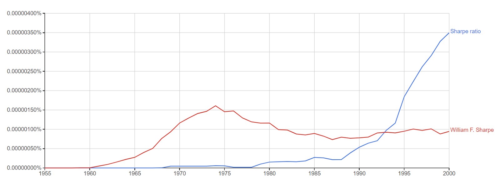
A Brief History of Sharpe Ratio, and Beyond
By James White and Victor Haghani 1
Early in the 1950s, academics and investors started proposing in earnest a variety of summary statistics to capture in a single number the quality of an investment. It was recognized that expected return wasn’t quite enough, because two investments with the same expected return could have dramatically different levels of risk. Pretty much everyone agreed that the quality statistic should be something like “expected return/risk”, but the devil was in the details, and especially in the definition of risk. In the 1960s, William Sharpe was a graduate student working with Harry Markowitz on Modern Portfolio Theory and the Capital Asset Pricing Model, work for which they’d later share a Nobel Prize along with Merton Miller. In 1966 Sharpe proposed a risk/reward ratio which he called the “reward-to-variability ratio,” or “R/V Ratio” 2 defined as:
Expected Return – Risk Free Rate Standard Deviation of Return
The name didn’t quite stick. Thirty years later, in a paper cheekily titled “The Sharpe Ratio”, 3 Sharpe himself concedes that his original term, which doesn’t exactly roll off the tongue, never gained popularity. Once he himself suggested referring to the measure as the “Sharpe Ratio,” the term as we know it today fell into common usage.
Though the original name wasn’t a hit, the concept was: a measure originally coined in the very specific context of a theoretical model came to be the de-facto standard amongst academics and investors for measuring the risk/reward quality of a wide variety of real-world investments.
Today use of Sharpe Ratio in both language and practice is ubiquitous, and naturally critiques of its use are nearly as ubiquitous. Some of the core critiques are:
- If Risk is taken to mean Risk of Loss, Standard Deviation and Risk are synonymous only when returns are Normally distributed. Many investments, such as corporate bonds, have asymmetric or fat-tailed return profiles, causing Sharpe Ratio to significantly mis-state the true riskiness of the investment.4
- Limited historical data can result in a Sharpe Ratio estimate which is significantly biased.5
Here we’d like to focus on a separate issue which arose from our note “Some Clarity on Risk Parity.” In that note, we said that if unlimited leverage is available to the investor at the risk-free rate, then the optimal portfolio from a risk-adjusted return standpoint will be the one with the best Sharpe Ratio, levered to give the optimal amount of expected return appropriate to the investor’s degree of risk-aversion. For many investors though, unlimited leverage on good terms isn’t feasible,6 either because the cost is higher than the risk-free rate, or because the investor just wants to avoid leverage.7
For the leverage-constrained investor, is Sharpe Ratio still all we need to look at to determine the best portfolio? As you’ve probably guessed, the answer is no: in the presence of leverage constraints, both Sharpe Ratio and the level of expected return are material factors in determining the portfolio with the best risk-adjusted return. In the chart below, we illustrate this in a simple two-asset case, showing the Sharpe Ratio and Risk-Adjusted Return from each possible combination of stocks and bonds, assuming the investor has a “typical” degree of risk aversion8 and her wealth is fully invested:9
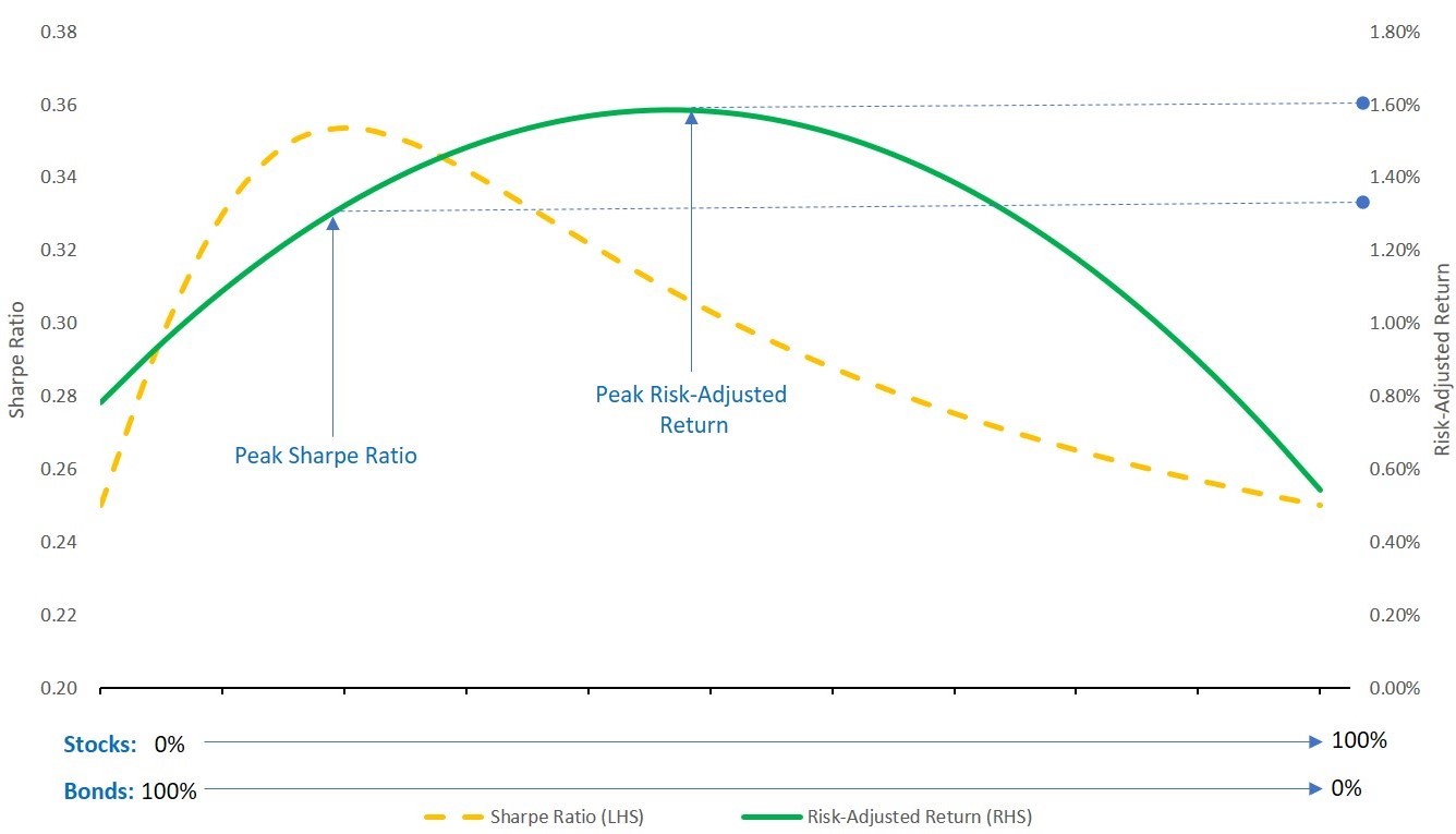
We can see that the portfolio with the best Sharpe Ratio is about 20%/80% Stocks/Bonds, but the portfolio with the best risk-adjusted return10 is about 45%/55% Stocks/Bonds.11 We believe allocating assets proportionally to risk-adjusted return is sound investing practice, and in the case of assets which follow a random-walk,12 risk-adjusted return is fortunately easy to calculate:
Risk-Adjusted Return = Expected Return – 1 2 γσ2
where γ is the investor’s level of risk-aversion and σ the asset’s volatility.
This relationship also gives us a formula for the trade-off between Sharpe Ratio and level of return given a leverage constraint. Consider our 45%/55% optimal un-levered portfolio from above – if instead of investing in this portfolio we were able to earn a higher expected return, but with a lower Sharpe Ratio, how much lower Sharpe Ratio could we bear and still be no worse off in terms of risk-adjusted return? The answer is:
SR* = R √ γ 2δ + γσ2
where SR* is the Sharpe Ratio which gives a fully-invested portfolio having return R* = R + δ the same risk-adjusted return as a portfolio with expected return R and volatility σ.
For a brief thought experiment, consider an asset with expected excess return of 4% and risk of 4% , for a (very good) Sharpe Ratio of 1. The risk-adjusted return of this asset is 3.78%13, and optimally, our portfolio allocation would greatly exceed 1, i.e. we’d optimally be highly levered. However, we have a leverage constraint, so instead we just hold our entire portfolio in this asset. Now we’re given the chance to switch into an alternative asset with a somewhat higher expected return of 4.5% – how much lower a Sharpe Ratio would we tolerate to still make the switch? The result is pretty surprising:
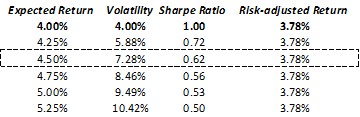
Here we have a list of hypothetical assets, all of which have the same risk-adjusted return, and we can clearly see the Expected Return/Sharpe Ratio trade-off at work – we’d switch to being fully invested in the 4.5% asset if its Sharpe Ratio is better than 0.62, a material discount from the reference portfolio Sharpe Ratio of 1.
Conclusion
As we can see from our thought experiment, in the presence of leverage constraints two portfolios with dramatically different Sharpe Ratios can be equally desirable. In the case of our stylized stock/bond example, the difference between the highest-Sharpe portfolio and the optimal portfolio is material but not too extreme – only about 0.25% per annum in risk-adjusted return. But this difference can be much bigger depending on your assumptions, especially if some of the assets involved have levered, asymmetric, or structured payouts. Our general point is that for most investors, and especially those with a desire to limit leverage, Sharpe Ratio is a useful and important metric, but doesn’t deliver the full-credit answer. To achieve the best expected risk-adjusted returns, investors with capital or leverage constraints need to think a step further, taking both Sharpe Ratio and the absolute level of their investments’ excess return into the mix.14
- This not is not an offer or solicitation to invest, nor should this be construed in any way as tax advice. Past returns are not indicative of future performance.
- Sharpe, William F. “Mutual Fund Performance”. Journal of Business, January 1966, pp. 119-138. (p. 123 in particular)
- William F. Sharpe, “The Sharpe Ratio”, Journal of Portfolio Management, 1994.
- Even relatively “vanilla” markets, such as the Broad US Equity market, can display markedly non-Normal behavior, especially over short to medium time-periods. Over longer time-periods this non-Normal behavior tends to lessen, though there’s still disagreement over whether Normal distributions are a sufficiently good model for long-term returns.
- Due to sampling error, survivorship bias and the critique above.
- Or accessing such leverage requires investing through 3rd-party managers with their own fee structures and potential agency issues.
- Consistent with a focus on capital preservation.
- We’ll define “typical” here as that degree of risk aversion that would maximize expected utility by investing 100% of savings in a stock/bond portfolio with a 60/40 mix. With our example numbers, this implies a coefficient of risk aversion in the Merton model of ~3 (2.7 is what we use in numerical examples throughout). For readers familiar with the Kelly Criterion, this means our investor is ~3x as risk averse as a Kelly bettor.
- We’re making a material assumption here that, in the absence of leverage, the investor optimally wants to be fully invested, vs. keeping part of her wealth in cash. That’s definitely not true in general, but in the case of our specific 2-asset example here, it is in fact true.
- In this context used interchangeably with “Expected Utility.”
- We assume that stocks and bonds can be described by un-correlated geometric Brownian motions, with stocks having 4% expected excess return and 16% volatility, and bonds having 1% expected excess return and 4% volatility.
- And investors with Constant-Relative-Risk-Aversion (CRRA) utility.
- Using the same risk-aversion as above.
- Your authors like the expected-utility framework for unifying these considerations within a single user-friendly toolkit, but we feel the specific method is less important than the general idea of translating expected returns into risk-adjusted returns before making your investment decisions.