By Victor Haghani and James White ¹

The Cyclically-Adjusted Price Earnings ratio, known as CAPE, is the most commonly used metric for estimating the long-term expected real return of the stock market. Although the merits of using cyclically-adjusted earnings were first suggested by Graham and Dodd in their magisterial book Security Analysis, Professors John Campbell and Robert Shiller share the primary credit for introducing the use of CAPE to forecast long-term stock market returns in their seminal 1988 research article “Stock Prices, Earnings, and Expected Dividends.”²

They suggested using a moving average of earnings “because yearly earnings are quite noisy as measures of fundamental value; they could even be negative while fundamental value cannot be negative.” And they concluded: “…we think that it can be argued that a long moving average of earnings is a very natural variable to use to represent fundamental value, and that there are not many competitors for this role.” While Campbell and Shiller used a 30-year moving average of earnings in their 1988 paper, over time, CAPE became defined as the price of an index of stocks divided by the index’s inflation-adjusted average earnings over the past ten years.

The reciprocal of CAPE (1/CAPE), known as the Cyclically-Adjusted Earnings Yield (CAEY), is the metric many investors use to estimate the long-term expected real return of the stock market. The rationale for this estimate is the supposition that, if companies paid out all their earnings to investors (whether as dividends or share buybacks), they would be able to maintain a constant level of real earnings in perpetuity – therefore, that earnings yield is also the expected real return. As we’ll see, this model of corporate earnings is not only appealing in terms of simplicity and intuition, but is also supported by the past 140 years of US public company experience, and is readily available for non-US equity markets over the shorter histories.

The chart below shows a common illustration of the relationship between CAEY and the next 10 years’ real return of the US stock market.

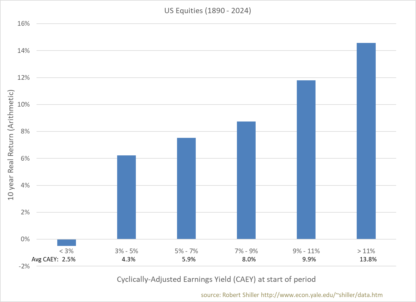
A shortcoming of Shiller and Campbell’s definition of cyclically-adjusted earnings is that it doesn’t take account of the fact that, in general, companies don’t pay out all their earnings as dividends each year. The fraction of earnings not paid out in dividends is either reinvested in the business or paid out via stock buybacks. Reinvesting earnings in the business is done in the expectation of growing future earnings, and this earnings growth should ideally be accounted for when smoothing earnings over the previous ten years for the purpose of predicting long-term future earnings. An empirical hint of why this might be an issue can be seen in the chart above, where using the traditional CAEY results in the average realized real return being about 1.5% higher than the average CAEY for the four central buckets.

To estimate how much retained earnings will grow future earnings, we prefer the use of cyclically-adjusted earnings yield rather than the default textbook metric of return on book equity. Return on book equity is a measure of the average return on equity in place, rather than the more relevant return on incremental equity – and, as an accounting metric, is subject to a variety of distortions. For example, book equity often ignores intangible assets (which have been growing rapidly as a fraction of total corporate assets in recent decades) and generally ignores upward mark-to-market on assets. Earnings yield (while imperfect) is, by contrast is a market-based signal – and empirically, it’s more consistent with historical earnings growth.

Buying back stock doesn’t grow top line earnings, but it does reduce shares outstanding and hence increases earnings per share. Again, the application of the market’s cyclically-adjusted earnings yield is the best simple estimate we have for how earnings used for stock buybacks will increase earnings per share over time.

To the extent that Campbell and Shiller’s definition of cyclically-adjusted earnings is meant to provide an estimate of future average earnings – smoothing out the peaks and troughs in the business cycle – then the measure really should take account of the dividend payout ratio, particularly when it is low. From 1880 to 1988, when Campbell and Shiller published their CAPE article, the average dividend payout ratio in the US was 65%, which perhaps wasn’t low enough to warrant an adjustment – but from 1988 to the end of 2024, the average dividend payout ratio fell to just 45%, and it’s dropped to 35% over the past two years.³

We believe a better measure of cyclically-adjusted earnings should directly account for the logic that retained earnings should increase earnings per share over time (whether through investment in the business or through share buybacks) in addition to the inflation adjustment already part of Campbell and Shiller’s measure. We believe such an adjustment is simple to implement and, when used to compute earnings yield, should provide a better measure of the long-term expected real return of the stock market. We call this modified measure “payout and cyclically-adjusted earnings,” or P-CAE. The earnings yield it’s used to compute we call “P-CAEY,” and the price-earnings multiple “P-CAPE.”

The way we compute payout and cyclically-adjusted earnings is to take each year’s inflation-adjusted earnings for the past ten years and bring forward the earnings not paid out as dividends at a growth rate equal to the CAEY at the time of those earnings.⁴ For example: if, ten years ago, the dividend payout ratio was 60%, real earnings on the stock market index were $10, and the CAEY was 6%, the payout-adjusted earnings we’d use would be:

60% * $10 + 40% * $10 * (1 + 6%)¹⁰ = $13.2

We then take the average of each of those ten years of payout and inflation-adjusted earnings.

Note that, for dividend payout ratios of less than 100% and for positive earnings yields, P-CAE will be higher than Shiller and Campbell’s cyclically-adjusted earnings, which are only adjusted for inflation. From 1890 to 2024, this new payout and cyclically-adjusted earnings metric was, on average, 19% higher than the standard cyclically-adjusted earnings metric.

How should we decide whether this is an improvement, and big enough to warrant its adoption? First and foremost, does it make sense? Doing something that has a stronger logical foundation is usually worth it, and we think this adjustment passes that first test. This is particularly important to think about before looking at the empirical results, as we just don’t have enough historical data to draw strong statistically-based conclusions.⁵

Second, with the caveat that 140 years of data isn’t that much when looking at 10-year stock market returns, we’ll want to compare how each metric has done in forecasting future earnings and returns.⁶ The table below shows a few summary statistics, which are supportive of the hypothesis that our suggested P-CAE metric is more useful than the same metric without the payout adjustment.

	Cyclically-Adjusted Earnings (CAE)	Payout AND Cyclically-Adjusted Earnings (P-CAE)
Window	10 years	10 years
Inflation-adjusted	Yes	Yes
Dividend Payout-Adjusted	No	Yes
	1890 – 2024 (full Shiller dataset)
Avg Cyclically-Adjusted Earnings vs Next Year’s Actual Earnings	-13%	2%
Average of Earnings Yield minus 10yr Prospective Market Real Return (Arithmetic per annum)	-1.4%	0.1%
% of Variance of 10yr Prospective Real Return Explained	24%	35%
	1950 – 2024 (post WWII)
Avg Cyclically-Adjusted Earnings vs Next Year’s Actual Earnings	-15%	0%
Average of Earnings Yield minus 10yr Prospective Market Real Return (Arithmetic per annum)	-1.9%	-0.5%
% of Variance of 10yr Prospective Real Return Explained	15%	33%

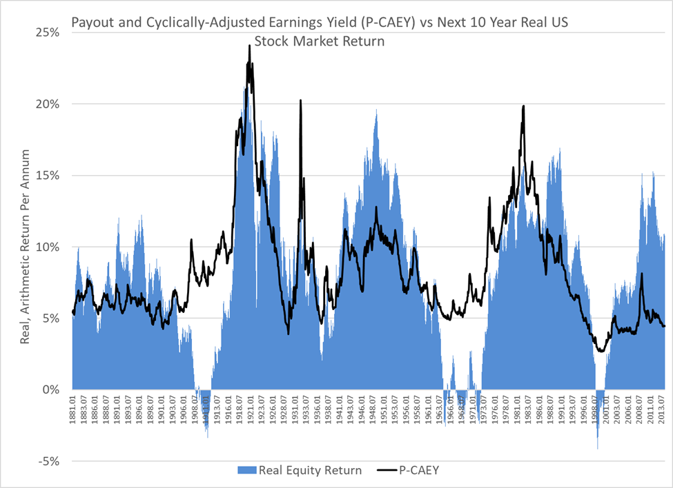
Notice that the standard Shiller and Campbell metric underestimates future earnings by 13% and 15% in the two periods, which we’d expect since that metric is not taking account of companies retaining earnings or repurchasing shares. Also, the shortfall is bigger in the more recent period, which is consistent with dividend payout ratios being lower over the second half of the 1890 – 2024 sample period. It’s also supportive that P-CAEY explains more of the next ten years of real returns, and by a decent margin in both samples.⁷ The chart below shows P-CAEY and the next ten-year US real stock market return.

Not adjusting for dividend payout rates leads to an increasingly poor raw earnings estimate as the window used for the estimate lengthens. For example: using the full US stock market earnings history from 1880 to 2024 as the window rather than ten years, Campbell and Shiller’s CAE would be $45 per S&P500 unit today, while the P-CAE estimate would be $210. Actual S&P500 earnings at the end of 2023 were $197.⁸ We are not suggesting that such a long window is preferable to a ten-year window, but rather to illustrate how the Shiller and Campbell metric diverges from the P-CAE suggested here, and it’s reassuring that P-CAE actually stands up pretty well to such a long window. It’s also comforting to note that the 2.1% annual rate of growth of US real corporate earnings experienced from 1890 to 2024 is what we’d expect from our simple model using an average dividend payout ratio of 65% and average growth rate of 6% on earnings not paid as dividends, assumptions which are not too far from actual experience.

Again, we must stress that the historical data available does not provide enough statistical power to make a decision solely on the basis of the data – but, if you’re already attracted to P-CAPE over CAPE based on the structural rationale, the empirical evidence does provide some further comfort.

In 2014, Bunn and Shiller suggested an adjustment to CAPE, which they called “Total Return CAPE (TR CAPE).” It adjusts for the changing dividend payout ratio over time. However, Bunn and Shiller’s TR CAPE makes its adjustment in such a way that in effect retained earnings are assumed to make future earnings lower, which is counter to economic logic. We believe that TR CAPE was constructed to be used as a statistical signal in a regression analysis context. In contrast, we are proposing P-CAEY as a direct forecast of the future real return of the stock market.

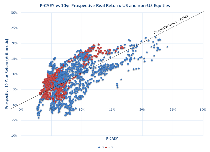
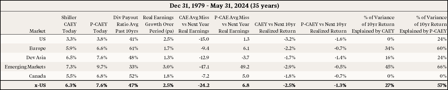
In the above analysis, we’ve used data graciously provided by Professor Shiller on his website. We have also studied the dividend payout adjustment using an alternative dataset for US stock market returns and earnings, and we’ve assessed non-US stock market datasets. We found results similar to those shown above, as can be seen in the table below. Another benefit of P-CAEY is that it gives a more consistent measure across international equity markets with different dividend payout ratios.

The one exception from a historical perspective has been the Canadian stock market. Neither CAEY nor P-CAEY has proven a useful return estimate over the past 35 years. Perhaps this is because Canada has had greater industry concentration than the other larger regional equity markets, or perhaps it’s due to 35 years of overlapping 10-year periods being such a sparse dataset.

We recognize that there are many who are critical of the use of CAEY as an estimator of future stock market real returns. We find most of these criticisms take the form of: “Twenty years ago, the CAEY of the US equity market was about 4.5% – but over the next 10 years, the actual was so much higher, coming in at 9.3% pa.”⁹ We don’t think the modification we’re suggesting in P-CAEY will go very far in changing the minds of such critics. We also think this isn’t a particularly valid criticism, as CAEY being a useful estimator doesn’t require that it explains all (or even most) long-term return variation. But, if you were attracted to the logic of Campbell and Shiller’s CAPE to begin with, we think you’ll find their measure adjusted for dividend payouts a worthwhile improvement.

---

Further Reading & References:

• Ang, A. and Bekaert, G. (2007), “Stock Return Predictability: Is it There?” Review of Financial Studies.
• Asness, C. (2012), “An Old Friend: The Stock Market’s Shiller P/E.” AQR.
• “Historic CAPE Ratio by country.” (2024). https://indices.cib.barclays/IM/21/en/indices/static/historic-cape.app Barclays.
• Boudoukh, J., Israel, R. and Richardson, M. (2019). “Long Horizon Predictability: A Cautionary Tale.” Financial Analysts Journal.
• Bunn, O., and Shiller, R. (2014). “Changing Times, Changing Values: A Historical Analysis of Sectors within the US Stock Market 1872-2013.” SSRN.
• Campbell, J. and Shiller, R. (1988). “Stock Prices, Earnings and Expected Dividends.” Journal of Finance.
• Campbell, J. and Thompson, S. (2007). “Predicting Excess Stock Returns Out of Sample: Can Anything Beat the Historical Average?” Review of Financial Studies.
• Cochrane, J. (1992). “Explaining the Variance of Price-Dividend Ratios.” Review of Financial Studies.
• Cochrane, J. (2011). “Presidential Address: Discount Rates.” Journal of Finance.
• Gavin, M. (2014). “Introducing the SCAPE: Why US equities are less expensive than they seem.” Barclays.
• Graham, B. and Dodd, D. (1934). Security Analysis. McGraw-Hill.
• Keimling, N. (2016). “Predicting Stock Market Returns Using the Shiller CAPE — An Improvement Towards Traditional Value Indicators?” SSRN.
• Shiller, R. and Jivraj, F. (2017). “The Many Colors of CAPE.” Barclays.
• Siegel, J. (2016). “The Shiller CAPE Ratio: A New Look.” Financial Analyst Journal.

---

1. This not is not an offer or solicitation to invest. Past returns are not indicative of future performance. Thank you to Larry Hilibrand, Vlad Ragulin, Samir Bouaoudia, Antti Ilmanen, John Campbell, Steve Mobbs, Andy Morton, Rich Dewey, Jeffrey Rosenbluth, Joshua Haghani and our partner Jerry Bell for reading drafts of this note and sharing their comments with us.
   
2. Graham and Dodd recommend an approach that “shifts the original point of departure, or basis of computation, from the current earnings to the average earnings, which should cover a period of not less than five years, and preferably seven to ten years.” (Security Analysis, page 452).
   
3. Some investment commentators like to estimate the long-term expected return of the stock market as the sum of current dividend yield plus expected dividend growth. The variability in corporate dividend policy over time poses a big challenge to that approach.
   
4. Ideally, we would like to use P-CAEY, reduced by .5 * σ² (σ = standard deviation of stock market returns) to convert from an arithmetic to a compound return. However, for simplicity and to avoid getting slightly different values as a function of the starting point, we use CAEY without the arithmetic-to-compound return adjustment.
   
5. Even if we assumed the data we have came from a stable distribution, which is almost certainly not the case.
   
6. Looking at monthly overlapping ten-year periods over 140 years has about the same statistical power as looking at just 14 to 17 back-to-back ten-year periods (far, far from the nearly 1,700 overlapping observations) depending on one’s assumptions about the underlying processes. See Boudoukh et al. (2019), “Long Horizon Predictability: A Cautionary Tale.”
   
7. We calculate “percent of variance explained” as 1 – f² / s² where f² is the average of the squared differences between CAEY (or P-CAEY) and realized real return, and s² is the variance of realized returns.
   
8. We view the small 7% difference as more of a coincidence than an argument for using a super-long window. Earnings from a century ago just don’t seem that relevant to estimating future earnings today.
   
9. There are many other criticisms to be sure, such as the arbitrary nature of the ten-year equal-weight window, and the failure to account for changing industry weights, but we think such criticisms are not the main ones. For a few examples of CAPE critiques, see: Armstrong, Robert. “The valuation mystery,” Financial Times, May 27, 2024, or Shah, Devesh. “Asset Allocation & International Equities, Part I: What is the right percentage allocation?” Mutual Fund Observer, June 2024.